Table of Contents
- I. COMPUTER NETWORKS
- 1. Distributed Algorithms
- 2. Network Simulation
- 14.1 Types of simulation
- 14.2 The need for communications network modelling and simulation
- 14.3 Types of communications networks, modelling constructs
- 14.4 Performance targets for simulation purposes
- 14.5 Traffic characterisation
- 14.6 Simulation modelling systems
- 14.7 Model Development Life Cycle (MDLC)
- 14.8 Modelling of traffic burstiness
- 14.9 Appendix A
- 3. Parallel Computations
- 4. Systolic Systems
- II. DATA BASES
- 5. Memory Management
- 6. Relational Database Design
- 7. Query Rewriting in Relational Databases
- 8. Semi-structured Databases
- III. APPLICATIONS
- 9. Bioinformatics
- 21.1 Algorithms on sequences
- 21.1.1 Distances of two sequences using linear gap penalty
- 21.1.2 Dynamic programming with arbitrary gap function
- 21.1.3 Gotoh algorithm for affine gap penalty
- 21.1.4 Concave gap penalty
- 21.1.5 Similarity of two sequences, the Smith-Waterman algorithm
- 21.1.6 Multiple sequence alignment
- 21.1.7 Memory-reduction with the Hirschberg algorithm
- 21.1.8 Memory-reduction with corner-cutting
- 21.2 Algorithms on trees
- 21.3 Algorithms on stochastic grammars
- 21.4 Comparing structures
- 21.5 Distance based algorithms for constructing evolutionary trees
- 21.6 Miscellaneous topics
- 10. Computer Graphics
- 11. Human-Computer Interaction
- Bibliography
 )-indexes
 )- and M(
 )-indexes
List of Figures
- 14.1. Estimation of the parameters of the most common distributions.
- 14.2. An example normal distribution.
- 14.3. An example Poisson distribution.
- 14.4. An example exponential distribution.
- 14.5. An example uniform distribution.
- 14.6. An example Pareto distribution.
- 14.7. Exponential distribution of interarrival time with 10 sec on the average.
- 14.8. Probability density function of the Exp (10.0) interarrival time.
- 14.9. Visualisation of anomalies in packet lengths.
- 14.10. Large deviations between delta times.
- 14.11. Histogram of frame lengths.
- 14.12. The three modelling abstraction levels specified by the Project, Node, and Process editors.
- 14.13. Example for graphical representation of scalar data (upper graph) and vector data (lower graph).
- 14.14. Figure 14.14 shows four graphs represented by the Analysis Tool.
- 14.15. Data Exchange Chart.
- 14.16. Summary of Delays.
- 14.17. Diagnosis window.
- 14.18. Statistics window.
- 14.19. Impact of adding more bandwidth on the response time.
- 14.20. Baseline model for further simulation studies.
- 14.21. Comparison of RMON Standards.
- 14.22. The self-similar nature of Internet network traffic.
- 14.23. Traffic traces.
- 14.24. Measured network parameters.
- 14.25. Part of the real network topology where the measurements were taken.
- 14.26. “Message Source” remote client.
- 14.27. Interarrival time and length of messages sent by the remote client.
- 14.28. The Pareto probability distribution for mean 440 bytes and Hurst parameter
 .
. - 14.29. The internal links of the 6Mbps ATM network with variable rate control (VBR).
- 14.30. Parameters of the 6Mbps ATM connection.
- 14.31. The “Destination” subnetwork.
- 14.32. utilisation of the frame relay link in the baseline model.
- 14.33. Baseline message delay between the remote client and the server.
- 14.34. Input buffer level of remote router.
- 14.35. Baseline utilisations of the DS-3 link and Ethernet link in the destination.
- 14.36. Network topology of bursty traffic sources with various Hurst parameters.
- 14.37. Simulated average and peak link utilisation.
- 14.38. Response time and burstiness.
- 14.39. Relation between the number of cells dropped and burstiness.
- 14.40. Utilisation of the frame relay link for fixed size messages.
- 14.41. Utilisation of the frame relay link for Hurst parameter
 .
. - 14.42. Utilisation of the frame relay link for Hurst parameter
 (many high peaks).
 - 14.43. Message delay for fixed size message.
- 14.44. Message delay for
 (longer response time peaks).
 - 14.45. Message delay for
 (extremely long response time peak).
 - 14.46. Settings.
- 14.47. New alert action.
- 14.48. Mailing information.
- 14.49. Settings.
- 14.50. Network topology.
- 15.1. SIMD architecture.
- 15.2. Bus-based SMP architecture.
- 15.3. ccNUMA architecture.
- 15.4. Ideal, typical, and super-linear speedup curves.
- 15.5. Locality optimisation by data transformation.
- 15.6. A simple MPI program.
- 15.7. Structure of an OpenMP program.
- 15.8. Matrix-vector multiply in OpenMP using a parallel loop.
- 15.9. Parallel random access machine.
- 15.10. Types of parallel random access machines.
- 15.11. A chain consisting of six processors.
- 15.12. A square of size
 .
. - 15.13. A 3-dimensional cube of size
 .
. - 15.14. A 4-dimensional hypercube
 .
. - 15.15. A butterfly model.
- 15.16. A ring consisting of 6 processors.
- 15.17. Computation of prefixes of 16 elements using
Optimal-Prefix. - 15.18. Input data of array ranking and the the result of the ranking.
- 15.19. Work of algorithm
Det-Rankingon the data of Example 15.4. - 15.20. Sorting of 16 numbers by algorithm
Odd-Even-Merge. - 15.21. A work-optimal merge algorithm
Optimal-Merge. - 15.22. Selection of maximal integer number.
- 15.23. Prefix computation on square.
- 16.1. Rectangular systolic array for matrix product. (a) Array structure and input scheme. (b) Cell structure.
- 16.2. Two snapshots for the systolic array from Figure 16.1.
- 16.3. Hexagonal systolic array for matrix product. (a) Array structure and principle of the data input/output. (b) Cell structure.
- 16.4. Image of a rectangular domain under projection. Most interior points have been suppressed for clarity. Images of previous vertex points are shaded.
- 16.5. Partitioning of the space coordinates.
- 16.6. Detailed input/output scheme for the systolic array from Figure 16.3(a).
- 16.7. Extended input/output scheme, correcting Figure 16.6.
- 16.8. Interleaved calculation of three matrix products on the systolic array from Figure 16.3.
- 16.9. Resetting registers via global control. (a) Array structure. (b) Cell structure.
- 16.10. Output scheme with delayed output of results.
- 16.11. Combined local/global control. (a) Array structure. (b) Cell structure.
- 16.12. Matrix product on a rectangular systolic array, with output of results and distributed control. (a) Array structure. (b) Cell structure.
- 16.13. Matrix product on a rectangular systolic array, with output of results and distributed control. (a) Array structure. (b) Cell on the upper border.
- 16.14. Bubble sort algorithm on a linear systolic array. (a) Array structure with input/output scheme. (b) Cell structure.
- 17.1. Task system
 , and its optimal schedule.
 - 17.2. Scheduling of the task system
 at list
  .
. - 17.3. Scheduling of the task system
 using list
  on
on  processors.
 - 17.4. Scheduling of
 with list
  on
on  processors.
 - 17.5. Scheduling task system
 on
on  processors.
 - 17.6. Task system
 and its optimal scheduling
  on two processors.
 - 17.7. Optimal list scheduling of task system
 .
. - 17.8. Scheduling
 belonging to list
  .
. - 17.9. Scheduling
 belonging to list
  .
. - 17.10. Identical graph of task systems
 and
and  .
. - 17.11. Schedulings
 and
and  .
. - 17.12. Graph of the task system
 .
. - 17.13. Optimal scheduling
 .
. - 17.14. Scheduling
 .
. - 17.15. Precedence graph of task system
 .
. - 17.16. The optimal scheduling
 (
( ,
,  ,
,  ).
). - 17.17. The optimal scheduling
 (
( ,
,  ,
,  ,
,  ,
,  ,
,  ).
). - 17.18. Summary of the numbers of discs.
- 17.19. Pairwise comparison of algorithms.
- 17.20. Results of the pairwise comparison of algorithms.
- 18.1. Application of
Join-test(
). - 19.1. The database CinePest.
- 19.2. The three levels of database architecture.
- 19.3. GMAPs for the university domain.
- 19.4. The graph
 .
. - 19.5. The graph
 .
. - 19.6. A taxonomy of work on answering queries using views.
- 20.1. Edge-labeled graph assigned to a vertex-labeled graph.
- 20.2. An edge-labeled graph and the corresponding vertex-labeled graph.
- 20.3. The graph corresponding to the XML file “forbidden”.
- 20.4. A relational database in the semi-structured model.
- 20.5. The schema of the semi-structured database given in Figure 20.4.
- 21.1. The tree on which we introduce the Felsenstein algorithm. Evolutionary times are denoted with
 s on the edges of the tree.
 - 21.2. A dendrogram.
- 21.3. Connecting leaf
 to the dendrogram.
 - 21.4. Calculating
 according to the
 Centroidmethod. - 21.5. Connecting leaf
 for constructing an additive tree.
 - 21.6. Some tree topologies for proving Theorem 21.7.
- 21.7. The configuration of nodes
 ,
,  ,
,  and
and  if
if  and
and  follows a cherry motif.
 - 21.8. The possible places for node
 on the tree.
 - 21.9. Representation of the
 signed permutation with an unsigned permutation, and its graph of desire and reality.
 - 22.1. Functions defining the sphere, the block, and the torus.
- 22.2. Parametric forms of the sphere, the cylinder, and the cone, where
![Parametric forms of the sphere, the cylinder, and the cone, where u,v\in[0,1] .](math/eq22_anon1137.png) .
. - 22.3. Parametric forms of the ellipse, the helix, and the line segment, where
![Parametric forms of the ellipse, the helix, and the line segment, where t\in[0,1] .](math/eq22_anon1156.png) .
. - 22.4. A Bézier curve defined by four control points and the respective basis functions (
 ).
). - 22.5. Construction of B-spline basis functions. A higher order basis function is obtained by blending two consecutive basis functions on the previous level using a linearly increasing and a linearly decreasing weighting, respectively. Here the number of control points is 5, i.e.
![Construction of B-spline basis functions. A higher order basis function is obtained by blending two consecutive basis functions on the previous level using a linearly increasing and a linearly decreasing weighting, respectively. Here the number of control points is 5, i.e. m=4 . Arrows indicate useful interval [t_{k-1},t_{m+1}] where we can find m+1 number of basis functions that add up to 1. The right side of the figure depicts control points with triangles and curve points corresponding to the knot values by circles.](math/eq22_anon1203.png) . Arrows indicate useful interval
. Arrows indicate useful interval ![Construction of B-spline basis functions. A higher order basis function is obtained by blending two consecutive basis functions on the previous level using a linearly increasing and a linearly decreasing weighting, respectively. Here the number of control points is 5, i.e. m=4 . Arrows indicate useful interval [t_{k-1},t_{m+1}] where we can find m+1 number of basis functions that add up to 1. The right side of the figure depicts control points with triangles and curve points corresponding to the knot values by circles.](math/eq22_anon1204.png) where we can find
where we can find ![Construction of B-spline basis functions. A higher order basis function is obtained by blending two consecutive basis functions on the previous level using a linearly increasing and a linearly decreasing weighting, respectively. Here the number of control points is 5, i.e. m=4 . Arrows indicate useful interval [t_{k-1},t_{m+1}] where we can find m+1 number of basis functions that add up to 1. The right side of the figure depicts control points with triangles and curve points corresponding to the knot values by circles.](math/eq22_anon1205.png) number of basis functions that add up to 1. The right side of the figure depicts control points with triangles and curve points corresponding to the knot values by circles.
number of basis functions that add up to 1. The right side of the figure depicts control points with triangles and curve points corresponding to the knot values by circles. - 22.6. A B-spline interpolation. Based on points
 to be interpolated, control points
  are computed to make the start and end points of the segments equal to the interpolated points.
 - 22.7. Iso-parametric curves of surface.
- 22.8. The influence decreases with the distance. Spheres of influence of similar signs increase, of different signs decrease each other.
- 22.9. The operations of constructive solid geometry for a cone of implicit function
 and for a sphere of implicit function
  : union (
 ), intersection (
 ), and difference (
 ).
). - 22.10. Constructing a complex solid by set operations. The root and the leaf of the CSG tree represents the complex solid, and the primitives, respectively. Other nodes define the set operations (U: union,
 : difference).
 - 22.11. Types of polygons. (a) simple; (b) complex, single connected; (c) multiply connected.
- 22.12. Diagonal and ear of a polygon.
- 22.13. The proof of the existence of a diagonal for simple polygons.
- 22.14. Tessellation of parametric surfaces.
- 22.15. Estimation of the tessellation error.
- 22.16. T vertices and their elimination with forced subdivision.
- 22.17. Construction of a subdivision curve: at each step midpoints are obtained, then the original vertices are moved to the weighted average of neighbouring midpoints and of the original vertex.
- 22.18. One smoothing step of the Catmull-Clark subdivision. First the face points are obtained, then the edge midpoints are moved, and finally the original vertices are refined according to the weighted sum of its neighbouring edge and face points.
- 22.19. Original mesh and its subdivision applying the smoothing step once, twice and three times, respectively.
- 22.20. Generation of the new edge point with butterfly subdivision.
- 22.21. Possible intersections of the per-voxel tri-linear implicit surface and the voxel edges. From the possible 256 cases, these 15 topologically different cases can be identified, from which the others can be obtained by rotations. Grid points where the implicit function has the same sign are depicted by circles.
- 22.22. Polyhedron-point containment test. A convex polyhedron contains a point if the point is on that side of each face plane where the polyhedron is. To test a concave polyhedron, a half line is cast from the point and the number of intersections is counted. If the result is an odd number, then the point is inside, otherwise it is outside.
- 22.23. Point in triangle containment test. The figure shows that case when point
 is on the left of oriented lines
  and
and  , and on the right of line
  , that is, when it is not inside the triangle.
 - 22.24. Point in triangle containment test on coordinate plane
 . Third vertex
  can be either on the left or on the right side of oriented line
  , which can always be traced back to the case of being on the left side by exchanging the vertices.
 - 22.25. Polyhedron-polyhedron collision detection. Only a part of collision cases can be recognized by testing the containment of the vertices of one object with respect to the other object. Collision can also occur when only edges meet, but vertices do not penetrate to the other object.
- 22.26. Clipping of simple convex polygon
![Clipping of simple convex polygon \vec{p}[0],\ldots,\vec{p}[5] results in polygon \vec{q}[0],\ldots,\vec{q}[4] . The vertices of the resulting polygon are the inner vertices of the original polygon and the intersections of the edges and the boundary plane.](math/eq22_anon1472.png) results in polygon
results in polygon ![Clipping of simple convex polygon \vec{p}[0],\ldots,\vec{p}[5] results in polygon \vec{q}[0],\ldots,\vec{q}[4] . The vertices of the resulting polygon are the inner vertices of the original polygon and the intersections of the edges and the boundary plane.](math/eq22_anon1473.png) . The vertices of the resulting polygon are the inner vertices of the original polygon and the intersections of the edges and the boundary plane.
. The vertices of the resulting polygon are the inner vertices of the original polygon and the intersections of the edges and the boundary plane. - 22.27. When concave polygons are clipped, the parts that should fall apart are connected by even number of edges.
- 22.28. The 4-bit codes of the points in a plane and the 6-bit codes of the points in space.
- 22.29. The embedded model of the projective plane: the projective plane is embedded into a three-dimensional Euclidean space, and a correspondence is established between points of the projective plane and lines of the embedding three-dimensional Euclidean space by fitting the line to the origin of the three-dimensional space and the given point.
- 22.30. Ray tracing.
- 22.31. Partitioning the virtual world by a uniform grid. The intersections of the ray and the coordinate planes of the grid are at regular distances
 ,
,  , and
, and  , respectively.
 - 22.32. Encapsulation of the intersection space by the cells of the data structure in a uniform subdivision scheme. The intersection space is a cylinder of radius
 . The candidate space is the union of those spheres that may overlap a cell intersected by the ray.
 - 22.33. A quadtree partitioning the plane, whose three-dimensional version is the octree. The tree is constructed by halving the cells along all coordinate axes until a cell contains “just a few” objects, or the cell sizes gets smaller than a threshold. Objects are registered in the leaves of the tree.
- 22.34. A kd-tree. A cell containing “many” objects are recursively subdivided to two cells with a plane that is perpendicular to one of the coordinate axes.
- 22.35. Notations and cases of algorithm
Ray-First-Intersection-with-kd-Tree. ,
,  , and
, and  are the ray parameters of the entry, exit, and the separating plane, respectively.
  is the signed distance between the ray origin and the separating plane.
 - 22.36. Kd-tree based space partitioning with empty space cutting.
- 22.37. Steps of incremental rendering. (a) Modelling defines objects in their reference state. (b) Shapes are tessellated to prepare for further processing. (c) Modelling transformation places the object in the world coordinate system. (d) Camera transformation translates and rotates the scene to get the eye to be at the origin and to look parallel with axis
 . (e) Perspective transformation converts projection lines meeting at the origin to parallel lines, that is, it maps the eye position onto an ideal point. (f) Clipping removes those shapes and shape parts, which cannot be projected onto the window. (g) Hidden surface elimination removes those surface parts that are occluded by other shapes. (h) Finally, the visible polygons are projected and their projections are filled with their visible colours.
 - 22.38. Parameters of the virtual camera: eye position
 , target
  , and vertical direction
  , from which camera basis vectors
  are obtained, front
  and back
  clipping planes, and vertical field of view
  (the horizontal field of view is computed from aspect ratio
  ).
). - 22.39. The normalizing transformation sets the field of view to 90 degrees.
- 22.40. The perspective transformation maps the finite frustum of pyramid defined by the front and back clipping planes, and the edges of the window onto an axis aligned, origin centred cube of edge size 2.
- 22.41. Notations of the Bresenham algorithm:
 is the signed distance between the closest pixel centre and the line segment along axis
  , which is positive if the line segment is above the pixel centre.
  is the distance along axis
  between the pixel centre just above the closest pixel and the line segment.
 - 22.42. Polygon fill. Pixels inside the polygon are identified scan line by scan line.
- 22.43. Incremental computation of the intersections between the scan lines and the edges. Coordinate
 always increases with the reciprocal of the slope of the line.
 - 22.44. The structure of the active edge table.
- 22.45. A triangle in the screen coordinate system. Pixels inside the projection of the triangle on plane
 need to be found. The
  coordinates of the triangle in these pixels are computed using the equation of the plane of the triangle.
 - 22.46. Incremental
 coordinate computation for a left oriented triangle.
 - 22.47. Polygon-window relations:: (a) distinct; (b) surrounding ; (c) intersecting; (d) contained.
- 22.48. A BSP-tree. The space is subdivided by the planes of the contained polygons.
- 23.1.
 shortest paths in a
  grid-graph, printed in overlap.
 - 23.2. The graph for Examples 23.1, 23.2 and 23.6.
- 23.3.
 for
for  on
on  grids.
 - 23.4. Example graph for the LP-penalty method.
- 23.5. An example for a non-unique decomposition in two paths.
- 23.6.
 for
for  on
on  grids.
|
AnTonCom, Budapest, 2011 This electronic book was prepared in the framework of project Eastern Hungarian Informatics Books Repository no. TÁMOP-4.1.2-08/1/A-2009-0046 This electronic book appeared with the support of European Union and with the co-financing of European Social Fund 
Editor: Antal Iványi Authors of Volume 1: László Lovász (Preface), Antal Iványi (Introduction), Zoltán Kása (Chapter 1), Zoltán Csörnyei (Chapter 2), Ulrich Tamm (Chapter 3), Péter Gács (Chapter 4), Gábor Ivanyos and Lajos Rónyai (Chapter 5), Antal Járai and Attila Kovács (Chapter 6), Jörg Rothe (Chapters 7 and 8), Csanád Imreh (Chapter 9), Ferenc Szidarovszky (Chapter 10), Zoltán Kása (Chapter 11), Aurél Galántai and András Jeney (Chapter 12) Validators of Volume 1: Zoltán Fülöp (Chapter 1), Pál Dömösi (Chapter 2), Sándor Fridli (Chapter 3), Anna Gál (Chapter 4), Attila Pethő (Chapter 5), Lajos Rónyai (Chapter 6), János Gonda (Chapter 7), Gábor Ivanyos (Chapter 8), Béla Vizvári (Chapter 9), János Mayer (Chapter 10), András Recski (Chapter 11), Tamás Szántai (Chapter 12), Anna Iványi (Bibliography) Authors of Volume 2: Burkhard Englert, Dariusz Kowalski, Gregorz Malewicz, and Alexander Shvartsman (Chapter 13), Tibor Gyires (Chapter 14), Claudia Fohry and Antal Iványi (Chapter 15), Eberhard Zehendner (Chapter 16), Ádám Balogh and Antal Iványi (Chapter 17), János Demetrovics and Attila Sali (Chapters 18 and 19), Attila Kiss (Chapter 20), István Miklós (Chapter 21), László Szirmay-Kalos (Chapter 22), Ingo Althöfer and Stefan Schwarz (Chapter 23) Validators of Volume 2: István Majzik (Chapter 13), János Sztrik (Chapter 14), Dezső Sima (Chapters 15 and 16), László Varga (Chapter 17), Attila Kiss (Chapters 18 and 19), András Benczúr (Chapter 20), István Katsányi (Chapter 21), János Vida (Chapter 22), Tamás Szántai (Chapter 23), Anna Iványi (Bibliography) ©2011 AnTonCom Infokommunikációs Kft. Homepage: http://www.antoncom.hu/ |
Table of Contents
- 1. Distributed Algorithms
- 2. Network Simulation
- 14.1 Types of simulation
- 14.2 The need for communications network modelling and simulation
- 14.3 Types of communications networks, modelling constructs
- 14.4 Performance targets for simulation purposes
- 14.5 Traffic characterisation
- 14.6 Simulation modelling systems
- 14.7 Model Development Life Cycle (MDLC)
- 14.8 Modelling of traffic burstiness
- 14.9 Appendix A
- 3. Parallel Computations
- 4. Systolic Systems
Table of Contents
We define a distributed system as a collection of individual computing devices that can communicate with each other. This definition is very broad, it includes anything, from a VLSI chip, to a tightly coupled multiprocessor, to a local area cluster of workstations, to the Internet. Here we focus on more loosely coupled systems. In a distributed system as we view it, each processor has its semi-independent agenda, but for various reasons, such as sharing of resources, availability, and fault-tolerance, processors need to coordinate their actions.
Distributed systems are highly desirable, but it is notoriously difficult to construct efficient distributed algorithms that perform well in realistic system settings. These difficulties are not just of a more practical nature, they are also fundamental in nature. In particular, many of the difficulties are introduced by the three factors of: asynchrony, limited local knowledge, and failures. Asynchrony means that global time may not be available, and that both absolute and relative times at which events take place at individual computing devices can often not be known precisely. Moreover, each computing device can only be aware of the information it receives, it has therefore an inherently local view of the global status of the system. Finally, computing devices and network components may fail independently, so that some remain functional while others do not.
We will begin by describing the models used to analyse distributed systems in the message-passing model of computation. We present and analyze selected distributed algorithms based on these models. We include a discussion of fault-tolerance in distributed systems and consider several algorithms for reaching agreement in the messages-passing models for settings prone to failures. Given that global time is often unavailable in distributed systems, we present approaches for providing logical time that allows one to reason about causality and consistent states in distributed systems. Moving on to more advanced topics, we present a spectrum of broadcast services often considered in distributed systems and present algorithms implementing these services. We also present advanced algorithms for rumor gathering algorithms. Finally, we also consider the mutual exclusion problem in the shared-memory model of distributed computation.
We present our first model of distributed computation, for message passing systems without failures. We consider both synchronous and asynchronous systems and present selected algorithms for message passing systems with arbitrary network topology, and both synchronous and asynchronous settings.
In a message passing system, processors communicate by sending messages over communication channels, where each channel provides a bidirectional connection between two specific processors. We call the pattern of connections described by the channels, the topology of the system. This topology is represented by an undirected graph, where each node represents a processor, and an edge is present between two nodes if and only if there is a channel between the two processors represented by the nodes. The collection of channels is also called the network. An algorithm for such a message passing system with a specific topology consists of a local program for each processor in the system. This local program provides the ability to the processor to perform local computations, to send and receive messages from each of its neighbours in the given topology.
Each processor in the system is modeled as a possibly infinite state machine. A configuration is a vector  where each
  is the state of a processor
  . Activities that can take place in the system are modeled as events (or actions) that describe indivisible system operations. Examples of events include local computation events and delivery events where a processor receives a message. The behaviour of the system over time is modeled as an execution, a (finite or infinite) sequence of configurations (
 ) alternating with events (
 ):
):  . Executions must satisfy a variety of conditions that are used to represent the correctness properties, depending on the system being modeled. These conditions can be classified as either safety or liveness conditions. A safety condition for a system is a condition that must hold in every finite prefix of any execution of the system. Informally it states that nothing bad has happened yet. A liveness condition is a condition that must hold a certain (possibly infinite) number of times. Informally it states that eventually something good must happen. An important liveness condition is fairness, which requires that an (infinite) execution contains infinitely many actions by a processor, unless after some configuration no actions are enabled at that processor.
We say that a system is asynchronous if there is no fixed upper bound on how long it takes for a message to be delivered or how much time elapses between consecutive steps of a processor. An obvious example of such an asynchronous system is the Internet. In an implementation of a distributed system there are often upper bounds on message delays and processor step times. But since these upper bounds are often very large and can change over time, it is often desirable to develop an algorithm that is independent of any timing parameters, that is, an asynchronous algorithm.
In the asynchronous model we say that an execution is admissible if each processor has an infinite number of computation events, and every message sent is eventually delivered. The first of these requirements models the fact that processors do not fail. (It does not mean that a processor's local program contains an infinite loop. An algorithm can still terminate by having a transition function not change a processors state after a certain point.)
We assume that each processor's set of states includes a subset of terminated states. Once a processor enters such a state it remains in it. The algorithm has terminated if all processors are in terminated states and no messages are in transit.
The message complexity of an algorithm in the asynchronous model is the maximum over all admissible executions of the algorithm, of the total number of (point-to-point) messages sent.
A timed execution is an execution that has a nonnegative real number associated with each event, the time at which the event occurs. To measure the time complexity of an asynchronous algorithm we first assume that the maximum message delay in any execution is one unit of time. Hence the time complexity is the maximum time until termination among all timed admissible executions in which every message delay is at most one. Intuitively this can be viewed as taking any execution of the algorithm and normalising it in such a way that the longest message delay becomes one unit of time.
In the synchronous model processors execute in lock-step. The execution is partitioned into rounds so that every processor can send a message to each neighbour, the messages are delivered, and every processor computes based on the messages just received. This model is very convenient for designing algorithms. Algorithms designed in this model can in many cases be automatically simulated to work in other, more realistic timing models.
In the synchronous model we say that an execution is admissible if it is infinite. From the round structure it follows then that every processor takes an infinite number of computation steps and that every message sent is eventually delivered. Hence in a synchronous system with no failures, once a (deterministic) algorithm has been fixed, the only relevant aspect determining an execution that can change is the initial configuration. On the other hand in an asynchronous system, there can be many different executions of the same algorithm, even with the same initial configuration and no failures, since here the interleaving of processor steps, and the message delays, are not fixed.
The notion of terminated states and the termination of the algorithm is defined in the same way as in the asynchronous model.
The message complexity of an algorithm in the synchronous model is the maximum over all admissible executions of the algorithm, of the total number of messages sent.
To measure time in a synchronous system we simply count the number of rounds until termination. Hence the time complexity of an algorithm in the synchronous model is the maximum number of rounds in any admissible execution of the algorithm until the algorithm has terminated.
We begin with some simple examples of algorithms in the message passing model.
We start with a simple algorithm Spanning-Tree-Broadcast for the (single message) broadcast problem, assuming that a spanning tree of the network graph with  nodes (processors) is already given. Later, we will remove this assumption. A processor
  wishes to send a message
  to all other processors. The spanning tree rooted at
  is maintained in a distributed fashion: Each processor has a distinguished channel that leads to its parent in the tree as well as a set of channels that lead to its children in the tree. The root
  sends the message
  on all channels leading to its children. When a processor receives the message on a channel from its parent, it sends
  on all channels leading to its children.
Spanning-Tree-Broadcast
Initiallyis in transit from
to all its children in the spanning tree. Code for
: 1 upon receiving no message: // first computation event by
2
TERMINATECode for,
,
: 3 upon receiving
from parent: 4
SENDto all children 5
TERMINATE
The algorithm Spanning-Tree-Broadcast is correct whether the system is synchronous or asynchronous. Moreover, the message and time complexities are the same in both models.
Using simple inductive arguments we will first prove a lemma that shows that by the end of round  , the message
  reaches all processors at distance
  (or less) from
  in the spanning tree.
Lemma 13.1 In every admissible execution of the broadcast algorithm in the synchronous model, every processor at distance  from
from  in the spanning tree receives the message
  in round
  .
.
Proof. We proceed by induction on the distance  of a processor from
  . First let
  . It follows from the algorithm that each child of
  receives the message in round 1.
Assume that each processor at distance  received the message
  in round
  . We need to show that each processor
  at distance
  receives the message in round
  . Let
. Let  be the parent of
  in the spanning tree. Since
  is at distance
  from
from  , by the induction hypothesis,
  received
  in round
  . By the algorithm,
  will hence receive
  in round
  .
.

By Lemma 13.1 the time complexity of the broadcast algorithm is  , where
  is the depth of the spanning tree. Now since
  is at most
  (when the spanning tree is a chain) we have:
Theorem 13.2 There is a synchronous broadcast algorithm for  processors with message complexity
  and time complexity
  , when a rooted spanning tree with depth
  is known in advance.
We now move to an asynchronous system and apply a similar analysis.
Lemma 13.3 In every admissible execution of the broadcast algorithm in the asynchronous model, every processor at distance  from
from  in the spanning tree receives the message
  by time
  .
.
We proceed by induction on the distance  of a processor from
  . First let
  . It follows from the algorithm that
  is initially in transit to each processor
  at distance
  from
from  . By the definition of time complexity for the asynchronous model,
  receives
  by time 1.
Assume that each processor at distance  received the message
  at time
  . We need to show that each processor
  at distance
  receives the message by time
  . Let
. Let  be the parent of
  in the spanning tree. Since
  is at distance
  from
from  , by the induction hypothesis,
  sends
sends  to
to  when it receives
  at time
  . By the algorithm,
  will hence receive
  by time
  .
.
We immediately obtain:
Theorem 13.4 There is an asynchronous broadcast algorithm for  processors with message complexity
  and time complexity
  , when a rooted spanning tree with depth
  is known in advance.
The asynchronous algorithm called Flood, discussed next, constructs a spanning tree rooted at a designated processor  . The algorithm is similar to the Depth First Search (DFS) algorithm. However, unlike DFS where there is just one processor with “global knowledge” about the graph, in the
 Flood algorithm, each processor has “local knowledge” about the graph, processors coordinate their work by exchanging messages, and processors and messages may get delayed arbitrarily. This makes the design and analysis of Flood algorithm challenging, because we need to show that the algorithm indeed constructs a spanning tree despite conspiratorial selection of these delays.
Each processor has four local variables. The links adjacent to a processor are identified with distinct numbers starting from 1 and stored in a local variable called  . We will say that the spanning tree has been constructed, when the variable parent stores the identifier of the link leading to the parent of the processor in the spanning tree, except that this variable is
 NONE for the designated processor  ; children is a set of identifiers of the links leading to the children processors in the tree; and other is a set of identifiers of all other links. So the knowledge about the spanning tree may be “distributed” across processors.
The code of each processor is composed of segments. There is a segment (lines 1–4) that describes how local variables of a processor are initialised. Recall that the local variables are initialised that way before time 0. The next three segments (lines 5–11, 12–15 and 16–19) describe the instructions that any processor executes in response to having received a message: <adopt>, <approved> or <rejected>. The last segment (lines 20–22) is only included in the code of processor  . This segment is executed only when the local variable parent of processor
  is
is NIL. At some point of time, it may happen that more than one segment can be executed by a processor (e.g., because the processor received <adopt> messages from two processors). Then the processor executes the segments serially, one by one (segments of any given processor are never executed concurrently). However, instructions of different processor may be arbitrarily interleaved during an execution. Every message that can be processed is eventually processed and every segment that can be executed is eventually executed (fairness).
Flood
Code for any processor,
1
INITIALISATION2 parent
NIL3 children4 other
5
PROCESS MESSAGE<adopt> that has arrived on link6
IFparentNIL7THENparent8
SEND<approved> to link9
SEND<adopt> to all links in neighbours10
ELSESEND<rejected> to link11
PROCESS MESSAGE<approved> that has arrived on link12 children
children
13
IFchildrenother
neighbours
{parent} 14
THENTERMINATE15PROCESS MESSAGE<rejected> that has arrived on link16 other
other
17
IFchildrenother
neighbours
{parent} 18
THENTERMINATEExtra code for the designated processor19
IFparentNIL20THENparentNONE21SEND<adopt> to all links in neighbours


Let us outline how the algorithm works. The designated processor sends an <adopt> message to all its neighbours, and assigns NONE to the parent variable (NIL and NONE are two distinguished values, different from any natural number), so that it never again sends the message to any neighbour.
When a processor processes message <adopt> for the first time, the processor assigns to its own parent variable the identifier of the link on which the message has arrived, responds with an <approved> message to that link, and forwards an <adopt> message to every other link. However, when a processor processes message <adopt> again, then the processor responds with a <rejected> message, because the parent variable is no longer NIL.
When a processor processes message <approved>, it adds the identifier of the link on which the message has arrived to the set children. It may turn out that the sets children and other combined form identifiers of all links adjacent to the processor except for the identifier stored in the parent variable. In this case the processor enters a terminating state.
When a processor processes message <rejected>, the identifier of the link is added to the set other. Again, when the union of children and other is large enough, the processor enters a terminating state.
We now argue that Flood constructs a spanning tree. The key moments in the execution of the algorithm are when any processor assigns a value to its parent variable. These assignments determine the “shape” of the spanning tree. The facts that any processor eventually executes an instruction, any message is eventually delivered, and any message is eventually processed, ensure that the knowledge about these assignments spreads to neighbours. Thus the algorithm is expanding a subtree of the graph, albeit the expansion may be slow. Eventually, a spanning tree is formed. Once a spanning tree has been constructed, eventually every processor will terminate, even though some processors may have terminated even before the spanning tree has been constructed.
Lemma 13.5 For any  , there is time
  which is the first moment when there are exactly
  processors whose parent variables are not
 NIL, and these processors and their parent variables form a tree rooted at  .
.
Proof. We prove the statement of the lemma by induction on  . For the base case, assume that
  . Observe that processor
  eventually assigns
 NONE to its parent variable. Let  be the moment when this assignment happens. At that time, the parent variable of any processor other than
  is still
 NIL, because no <adopt> messages have been sent so far. Processor  and its parent variable form a tree with a single node and not arcs. Hence they form a rooted tree. Thus the inductive hypothesis holds for
  .
.
For the inductive step, suppose that  and that the inductive hypothesis holds for
  . Consider the time
  which is the first moment when there are exactly
  processors whose parent variables are not
 NIL. Because  , there is a non-tree processor. But the graph
  is connected, so there is a non-tree processor adjacent to the tree. (For any subset
  of processors, a processor
  is adjacent to
  if and only if there an edge in the graph
  from
from  to a processor in
  .) Recall that by definition, parent variable of such processor is
 NIL. By the inductive hypothesis, the  processors must have executed line
  of their code, and so each either has already sent or will eventually send <adopt> message to all its neighbours on links other than the parent link. So the non-tree processors adjacent to the tree have already received or will eventually receive <adopt> messages. Eventually, each of these adjacent processors will, therefore, assign a value other than
 NIL to its parent variable. Let  be the first moment when any processor performs such assignment, and let us denote this processor by
  . This cannot be a tree processor, because such processor never again assigns any value to its parent variable. Could
  be a non-tree processor that is not adjacent to the tree? It could not, because such processor does not have a direct link to a tree processor, so it cannot receive <adopt> directly from the tree, and so this would mean that at some time
  between
  and
and  some other non-tree processor
  must have sent <adopt> message to
  , and so
  would have to assign a value other than
 NIL to its parent variable some time after  but before
  , contradicting the fact the
  is the first such moment. Consequently,
  is a non-tree processor adjacent to the tree, such that, at time
  ,
,  assigns to its parent variable the index of a link leading to a tree processor. Therefore, time
  is the first moment when there are exactly
  processors whose parent variables are not
 NIL, and, at that time, these processors and their parent variables form a tree rooted at  . This completes the inductive step, and the proof of the lemma.
Theorem 13.6 Eventually each processor terminates, and when every processor has terminated, the subgraph induced by the parent variables forms a spanning tree rooted at  .
.
Proof. By Lemma 13.5, we know that there is a moment  which is the first moment when all processors and their parent variables form a spanning tree.
Is it possible that every processor has terminated before time  ? By inspecting the code, we see that a processor terminates only after it has received <rejected> or <approved> messages from all its neighbours other than the one to which parent link leads. A processor receives such messages only in response to <adopt> messages that the processor sends. At time
  , there is a processor that still has not even sent <adopt> messages. Hence, not every processor has terminated by time
  .
.
Will every processor eventually terminate? We notice that by time  , each processor either has already sent or will eventually send <adopt> message to all its neighbours other than the one to which parent link leads. Whenever a processor receives <adopt> message, the processor responds with <rejected> or <approved>, even if the processor has already terminated. Hence, eventually, each processor will receive either <rejected> or <approved> message on each link to which the processor has sent <adopt> message. Thus, eventually, each processor terminates.
We note that the fact that a processor has terminated does not mean that a spanning tree has already been constructed. In fact, it may happen that processors in a different part of the network have not even received any message, let alone terminated.
Theorem 13.7 Message complexity of Flood is  , where
  is the number of edges in the graph
  .
.
The proof of this theorem is left as Problem 13-1.
Exercises
13.2-1 It may happen that a processor has terminated even though a processor has not even received any message. Show a simple network and how to delay message delivery and processor computation to demonstrate that this can indeed happen.
13.2-2 It may happen that a processor has terminated but may still respond to a message. Show a simple network and how to delay message delivery and processor computation to demonstrate that this can indeed happen.
One often needs to coordinate the activities of processors in a distributed system. This can frequently be simplified when there is a single processor that acts as a coordinator. Initially, the system may not have any coordinator, or an existing coordinator may fail and so another may need to be elected. This creates the problem where processors must elect exactly one among them, a leader. In this section we study the problem for special types of networks—rings. We will develop an asynchronous algorithm for the problem. As we shall demonstrate, the algorithm has asymptotically optimal message complexity. In the current section, we will see a distributed analogue of the well-known divide-and-conquer technique often used in sequential algorithms to keep their time complexity low. The technique used in distributed systems helps reduce the message complexity.
The leader election problem is to elect exactly leader among a set of processors. Formally each processor has a local variable leader initially equal to NIL. An algorithm is said to solve the leader election problem if it satisfies the following conditions:
-
in any execution, exactly one processor eventually assigns
TRUEto its leader variable, all other processors eventually assignFALSEto their leader variables, and -
in any execution, once a processor has assigned a value to its leader variable, the variable remains unchanged.
We study the leader election problem on a special type of network—the ring. Formally, the graph  that models a distributed system consists of
  nodes that form a simple cycle; no other edges exist in the graph. The two links adjacent to a processor are labeled CW (Clock-Wise) and CCW (Counter Clock-Wise). Processors agree on the orientation of the ring i.e., if a message is passed on in CW direction
  times, then it visits all
  processors and comes back to the one that initially sent the message; same for CCW direction. Each processor has a unique identifier that is a natural number, i.e., the identifier of each processor is different from the identifier of any other processor; the identifiers do not have to be consecutive numbers
  . Initially, no processor knows the identifier of any other processor. Also processors do not know the size
  of the ring.
Bully elects a leader among asynchronous processors  . Identifiers of processors are used by the algorithm in a crucial way. Briefly speaking, each processor tries to become the leader, the processor that has the largest identifier among all processors blocks the attempts of other processors, declares itself to be the leader, and forces others to declare themselves not to be leaders.
Let us begin with a simpler version of the algorithm to exemplify some of the ideas of the algorithm. Suppose that each processor sends a message around the ring containing the identifier of the processor. Any processor passes on such message only if the identifier that the message carries is strictly larger than the identifier of the processor. Thus the message sent by the processor that has the largest identifier among the processors of the ring, will always be passed on, and so it will eventually travel around the ring and come back to the processor that initially sent it. The processor can detect that such message has come back, because no other processor sends a message with this identifier (identifiers are distinct). We observe that, no other message will make it all around the ring, because the processor with the largest identifier will not pass it on. We could say that the processor with the largest identifier “swallows” these messages that carry smaller identifiers. Then the processor becomes the leader and sends a special message around the ring forcing all others to decide not to be leaders. The algorithm has  message complexity, because each processor induces at most
  messages, and the leader induces
  extra messages; and one can assign identifiers to processors and delay processors and messages in such a way that the messages sent by a constant fraction of
  processors are passed on around the ring for a constant fraction of
  hops. The algorithm can be improved so as to reduce message complexity to
  , and such improved algorithm will be presented in the remainder of the section.
The key idea of the Bully algorithm is to make sure that not too many messages travel far, which will ensure  message complexity. Specifically, the activity of any processor is divided into phases. At the beginning of a phase, a processor sends “probe” messages in both directions: CW and CCW. These messages carry the identifier of the sender and a certain “time-to-live” value that limits the number of hops that each message can make. The probe message may be passed on by a processor provided that the identifier carried by the message is larger than the identifier of the processor. When the message reaches the limit, and has not been swallowed, then it is “bounced back”. Hence when the initial sender receives two bounced back messages, each from each direction, then the processor is certain that there is no processor with larger identifier up until the limit in CW nor CCW directions, because otherwise such processor would swallow a probe message. Only then does the processor enter the next phase through sending probe messages again, this time with the time-to-live value increased by a factor, in an attempt to find if there is no processor with a larger identifier in twice as large neighbourhood. As a result, a probe message that the processor sends will make many hops only when there is no processor with larger identifier in a large neighbourhood of the processor. Therefore, fewer and fewer processors send messages that can travel longer and longer distances. Consequently, as we will soon argue in detail, message complexity of the algorithm is
  .
.
We detail the Bully algorithm. Each processor has five local variables. The variable id stores the unique identifier of the processor. The variable leader stores TRUE when the processor decides to be the leader, and FALSE when it decides not to be the leader. The remaining three variables are used for bookkeeping: asleep determines if the processor has ever sent a <probe,id,0,0> message that carries the identifier id of the processor. Any processor may send <probe,id,phase,  > message in both directions (CW and CCW) for different values of phase. Each time a message is sent, a <reply,id,phase> message may be sent back to the processor. The variables
  and
and  are used to remember whether the replies have already been processed the processor.
The code of each processor is composed of five segments. The first segment (lines 1–5) initialises the local variables of the processor. The second segment (lines 6–8) can only be executed when the local variable asleep is TRUE. The remaining three segments (lines 9–17, 1–26, and 27–31) describe the actions that the processor takes when it processes each of the three types of messages: <probe,ids,phase,ttl>, <reply,ids,phase> and <terminate> respectively. The messages carry parameters  , phase and
  that are natural numbers.
We now describe how the algorithm works. Recall that we assume that the local variables of each processor have been initialised before time 0 of the global clock. Each processor eventually sends a <probe,id,0,0> message carrying the identifier id of the processor. At that time we say that the processor enters phase number zero. In general, when a processor sends a message <probe,id,phase,  >, we say that the processor enters phase number phase. Message <probe,id,0,0> is never sent again because
 FALSE is assigned to asleep in line 7. It may happen that by the time this message is sent, some other messages have already been processed by the processor.
When a processor processes message <probe,ids,phase,ttl> that has arrived on link CW (the link leading in the clock-wise direction), then the actions depend on the relationship between the parameter  and the identifier id of the processor. If
  is smaller than id, then the processor does nothing else (the processor swallows the message). If
  is equal to id and processor has not yet decided, then, as we shall see, the probe message that the processor sent has circulated around the entire ring. Then the processor sends a <terminate> message, decides to be the leader, and terminates (the processor may still process messages after termination). If
  is larger than id, then actions of the processor depend on the value of the parameter
  (time-to-live). When the value is strictly larger than zero, then the processor passes on the probe message with
  decreased by one. If, however, the value of
  is already zero, then the processor sends back (in the CW direction) a reply message. Symmetric actions are executed when the <</sl>probe,ids,phase,ttl</sl>> message has arrived on link CCW, in the sense that the directions of sending messages are respectively reversed – see the code for details.
Bully
Code for any processor,
1
INITIALISATION2 asleepTRUE3 CWrepliedFALSE4 CCWrepliedFALSE5 leaderNIL6IFasleep 7THENasleepFALSE8SEND<probe,id,0,0> to links CW and CCW 9PROCESS MESSAGE<probe,ids,phase,ttl> that has arrived on link CW (resp. CCW) 10IFidids and leader
NIL11THENSEND<terminate> to link CCW 12 leaderTRUE13TERMINATE14IFidsid and ttl
15
THENSEND<probe,ids,phase,ttl> to link CCW (resp. CW) 16
IFidsid and ttl
17
THENSEND<reply,ids,phase> to link CW (resp. CCW) 18PROCESS MESSAGE<reply,ids,phase> that has arrived on link CW (resp. CCW) 19IFidids 20
THENSEND<reply,ids,phase> to link CCW (resp. CW) 21ELSECWrepliedTRUE(resp. CCWreplied) 22IFCWreplied and CCWreplied 23THENCWrepliedFALSE24 CCWrepliedFALSE25SEND<probe,id,phase+1,> to links CW and CCW 26
PROCESS MESSAGE<terminate> that has arrived on link CW 27IFleaderNIL28THENSEND<terminate> to link CCW 29 leaderFALSE30TERMINATE


When a processor processes message <reply,ids,phase> that has arrived on link CW, then the processor first checks if ids is different from the identifier id of the processor. If so, the processor merely passes on the message. However, if  , then the processor records the fact that a reply has been received from direction CW, by assigning
 TRUE to CWreplied. Next the processor checks if both CWreplied and CCWreplied variables are true. If so, the processor has received replies from both directions. Then the processor assigns false to both variables. Next the processor sends a probe message. This message carries the identifier id of the processor, the next phase number  , and an increased time-to-live parameter
  . Symmetric actions are executed when <reply,ids,phase> has arrived on link CCW.
The last type of message that a processor can process is <terminate>. The processor checks if it has already decided to be or not to be the leader. When no decision has been made so far, the processor passes on the <terminate> message and decides not to be the leader. This message eventually reaches a processor that has already decided, and then the message is no longer passed on.
We begin the analysis by showing that the algorithm Bully solves the leader election problem.
Theorem 13.8 Bully solves the leader election problem on any ring with asynchronous processors.
Proof. We need to show that the two conditions listed at the beginning of the section are satisfied. The key idea that simplifies the argument is to focus on one processor. Consider the processor  with maximum id among all processors in the ring. This processor eventually executes lines 6–8. Then the processor sends <probe,id,0,0> messages in CW and CCW directions. Note that whenever the processor sends <probe,id,phase,
  > messages, each such message is always passed on by other processors, until the ttl parameter of the message drops down to zero, or the message travels around the entire ring and arrives at
  . If the message never arrives at
  , then a processor eventually receives the probe message with ttl equal to zero, and the processor sends a response back to
  . Then, eventually
  receives messages <reply,id,phase> from each directions, and enters phase number
  by sending probe messages <probe,id,phase+1,
  > in both directions. These messages carry a larger time-to-live value compared to the value from the previous phase number phase. Since the ring is finite, eventually ttl becomes so large that processor
  receives a probe message that carries the identifier of
  . Note that
  will eventually receive two such messages. The first time when
  processes such message, the processor sends a <terminate> message and terminates as the leader. The second time when
  processes such message, lines 11–13 are not executed, because variable leader is no longer
 NIL. Note that no other processor  can execute lines 11–13, because a probe message originated at
  cannot travel around the entire ring, since
  is on the way, and
  would swallow the message; and since identifiers are distinct, no other processor sends a probe message that carries the identifier of processor
  . Thus no processor other than
  can assign
 TRUE to its leader variable. Any processor other than  will receive the <terminate> message, assign
 FALSE to its leader variable, and pass on the message. Finally, the <terminate> message will arrive at  , and
, and  will not pass it anymore. The argument presented thus far ensures that eventually exactly one processor assigns
 TRUE to its leader variable, all other processors assign FALSE to their leader variables, and once a processor has assigned a value to its leader variable, the variable remains unchanged.
Our next task is to give an upper bound on the number of messages sent by the algorithm. The subsequent lemma shows that the number of processors that can enter a phase decays exponentially as the phase number increases.
Lemma 13.9 Given a ring of size  , the number
  of processors that enter phase number
  is at most
  .
.
Proof. There are exactly  processors that enter phase number
  , because each processor eventually sends <probe,id,0,0> message. The bound stated in the lemma says that the number of processors that enter phase 0 is at most
  , so the bound evidently holds for
  . Let us consider any of the remaining cases i.e., let us assume that
  . Suppose that a processor
  enters phase number
  , and so by definition it sends message <probe,id,i,
  >. In order for a processor to send such message, each of the two probe messages <probe,id,i-1,
  > that the processor sent in the previous phase in both directions must have made
  hops always arriving at a processor with strictly lower identifier than the identifier of
  (because otherwise, if a probe message arrives at a processor with strictly larger or the same identifier, than the message is swallowed, and so a reply message is not generated, and consequently
  cannot enter phase number
  ). As a result, if a processor enters phase number
  , then there is no other processor
  hops away in both directions that can ever enter the phase. Suppose that there are
  processors that enter phase
  . We can associate with each such processor
  , the
, the  consecutive processors that follow
  in the CW direction. This association assigns
  distinct processors to each of the
  processors. So there must be at least
  distinct processor in the ring. Hence
  , and so we can weaken this bound by dropping
  , and conclude that
  , as desired.
Theorem 13.10 The algorithm Bully has  message complexity, where
  is the size of the ring.
Note that any processor in phase  , sends messages that are intended to travel
  away and back in each direction (CW and CCW). This contributes at most
  messages per processor that enters phase number
  . The contribution may be smaller than
  if a probe message gets swallowed on the way away from the processor. Lemma 13.9 provides an upper bound on the number of processors that enter phase number
  . What is the highest phase that a processor can ever enter? The number
  of processors that can be in phase
  is at most
  . So when
  , then there can be no processor that ever enters phase
  . Thus no processor can enter any phase beyond phase number
  , because
  . Finally, a single processor sends one termination message that travels around the ring once. So for the total number of messages sent by the algorithm we get the
upper bound.
Burns furthermore showed that the asynchronous leader election algorithm is asymptotically optimal: Any uniform algorithm solving the leader election problem in an asynchronous ring must send the number of messages at least proportional to  .
.
Theorem 13.11 Any uniform algorithm for electing a leader in an asynchronous ring sends  messages.
The proof, for any algorithm, is based on constructing certain executions of the algorithm on rings of size  . Then two rings of size
  are pasted together in such a way that the constructed executions on the smaller rings are combined, and
  additional messages are received. This construction strategy yields the desired logarithmic multiplicative overhead.
Exercises
13.3-1 Show that the simplified Bully algorithm has  message complexity, by appropriately assigning identifiers to processors on a ring of size
  , and by determining how to delay processors and messages.
13.3-2 Show that the algorithm Bully has  message complexity.
The algorithms presented so far are based on the assumption that the system on which they run is reliable. Here we present selected algorithms for unreliable distributed systems, where the active (or correct) processors need to coordinate their activities based on common decisions.
It is inherently difficult for processors to reach agreement in a distributed setting prone to failures. Consider the deceptively simple problem of two failure-free processors attempting to agree on a common bit using a communication medium where messages may be lost. This problem is known as the two generals problem. Here two generals must coordinate an attack using couriers that may be destroyed by the enemy. It turns out that it is not possible to solve this problem using a finite number of messages. We prove this fact by contradiction. Assume that there is a protocol used by processors  and
and  involving a finite number of messages. Let us consider such a protocol that uses the smallest number of messages, say
  messages. Assume without loss of generality that the last
  message is sent from
  to
to  . Since this final message is not acknowledged by
  ,
,  must determine the decision value whether or not
  receives this message. Since the message may be lost,
  must determine the decision value without receiving this final message. But now both
  and
and  decide on a common value without needing the
  message. In other words, there is a protocol that uses only
  messages for the problem. But this contradicts the assumption that
  is the smallest number of messages needed to solve the problem.
In the rest of this section we consider agreement problems where the communication medium is reliable, but where the processors are subject to two types of failures: crash failures, where a processor stops and does not perform any further actions, and Byzantine failures, where a processor may exhibit arbitrary, or even malicious, behaviour as the result of the failure. The algorithms presented deal with the so called consensus problem, first introduced by Lamport, Pease, and Shostak. The consensus problem is a fundamental coordination problem that requires processors to agree on a common output, based on their possibly conflicting inputs.
We consider a system in which each processor  has a special state component
  , called the input and
  , called the output (also called the decision). The variable
  initially holds a value from some well ordered set of possible inputs and
  is undefined. Once an assignment to
  has been made, it is irreversible. Any solution to the consensus problem must guarantee:
-
Termination: In every admissible execution,
 is eventually assigned a value, for every nonfaulty processor
  .
. -
Agreement: In every execution, if
 and
and  are assigned, then
  , for all nonfaulty processors
  and
and  . That is nonfaulty processors do not decide on conflicting values.
 -
Validity: In every execution, if for some value
 ,
,  for all processors
  , and if
  is assigned for some nonfaulty processor
  , then
  . That is, if all processors have the same input value, then any value decided upon must be that common input.
Note that in the case of crash failures this validity condition is equivalent to requiring that every nonfaulty decision value is the input of some processor. Once a processor crashes it is of no interest to the algorithm, and no requirements are put on its decision.
We begin by presenting a simple algorithm for consensus in a synchronous message passing system with crash failures.
Since the system is synchronous, an execution of the system consists of a series of rounds. Each round consists of the delivery of all messages, followed by one computation event for every processor. The set of faulty processors can be different in different executions, that is, it is not known in advance. Let  be a subset of at most
  processors, the faulty processors. Each round contains exactly one computation event for the processors not in
  and at most one computation event for every processor in
  . Moreover, if a processor in
  does not have a computation event in some round, it does not have such an event in any further round. In the last round in which a faulty processor has a computation event, an arbitrary subset of its outgoing messages are delivered.
Consensus-with-Crash-Failures
Code for processor,
. Initially
round
,
1
SEND{has not already sent
} to all processors 2
RECEIVEfrom
,
,
3
4
IF5
THEN
In the previous algorithm, which is based on an algorithm by Dolev and Strong, each processor maintains a set of the values it knows to exist in the system. Initially, the set contains only its own input. In later rounds the processor updates its set by joining it with the sets received from other processors. It then broadcasts any new additions to the set of all processors. This continues for  rounds, where
  is the maximum number of processors that can fail. At this point, the processor decides on the smallest value in its set of values.
To prove the correctness of this algorithm we first notice that the algorithm requires exactly  rounds. This implies termination. Moreover the validity condition is clearly satisfied since the decision value is the input of some processor. It remains to show that the agreement condition holds. We prove the following lemma:
Lemma 13.12 In every execution at the end of round  ,
,  , for every two nonfaulty processors
  and
and  .
.
Proof. We prove the claim by showing that if  at the end of round
  then
then  at the end of round
  .
.
Let  be the first round in which
  is added to
  for any nonfaulty processor
  . If
. If  is initially in
  let
let  . If
. If  then, in round
 sends
sends  to each
  , causing
  to add
  to
to  , if not already present.
Otherwise, suppose  and let
  be a nonfaulty processor that receives
  for the first time in round
  . Then there must be a chain of
  processors
  that transfers the value
  to
to  . Hence
  sends
sends  to
to  in round one etc. until
  sends
sends  to
to  in round
  . But then
  is a chain of
  processors. Hence at least one of them, say
  must be nonfaulty. Hence
  adds
adds  to its set in round
  , contradicting the minimality of
  .
.
This lemma together with the before mentioned observations hence implies the following theorem.
Theorem 13.13 The previous consensus algorithm solves the consensus problem in the presence of  crash failures in a message passing system in
  rounds.
The following theorem was first proved by Fischer and Lynch for Byzantine failures. Dolev and Strong later extended it to crash failures. The theorem shows that the previous algorithm, assuming the given model, is optimal.
Theorem 13.14 There is no algorithm which solves the consensus problem in less than  rounds in the presence of
  crash failures, if
  .
.
What if failures are not benign? That is can the consensus problem be solved in the presence of Byzantine failures? And if so, how?
In a computation step of a faulty processor in the Byzantine model, the new state of the processor and the message sent are completely unconstrained. As in the reliable case, every processor takes a computation step in every round and every message sent is delivered in that round. Hence a faulty processor can behave arbitrarily and even maliciously. For example, it could send different messages to different processors. It can even appear that the faulty processors coordinate with each other. A faulty processor can also mimic the behaviour of a crashed processor by failing to send any messages from some point on.
In this case, the definition of the consensus problem is the same as in the message passing model with crash failures. The validity condition in this model, however, is not equivalent with requiring that every nonfaulty decision value is the input of some processor. Like in the crash case, no conditions are put on the output of faulty processors.
Pease, Shostak and Lamport first proved the following theorem.
Theorem 13.15 In a system with  processors and
  Byzantine processors, there is no algorithm which solves the consensus problem if
  .
.
The following algorithm uses messages of constant size, takes  rounds, and assumes that
  . It was presented by Berman and Garay.
This consensus algorithm for Byzantine failures contains  phases, each taking two rounds. Each processor has a preferred decision for each phase, initially its input value. At the first round of each phase, processors send their preferences to each other. Let
  be the majority value in the set of values received by processor
  at the end of the first round of phase
  . If no majority exists, a default value
  is used. In the second round of the phase processor
  , called the king of the phase, sends its majority value
  to all processors. If
  receives more than
  copies of
  (in the first round of the phase) then it sets its preference for the next phase to be
  ; otherwise it sets its preference to the phase kings preference,
  received in the second round of the phase. After
  phases, the processor decides on its preference. Each processor maintains a local array pref with
  entries.
We prove correctness using the following lemmas. Termination is immediate. We next note the persistence of agreement:
Lemma 13.16 If all nonfaulty processors prefer  at the beginning of phase
  , then they all prefer
  at the end of phase
  , for all
  ,
,  .
.
Proof. Since all nonfaulty processors prefer  at the beginning of phase
  , they all receive at least
  copies of
  (including their own) in the first round of phase
  . Since
  ,
,  , implying that all nonfaulty processors will prefer
  at the end of phase
  .
.
Consensus-with-Byzantine-failures
Code for processor,
. Initially
, for any
round
,
1
SENDto all processors 2
RECEIVEfrom
and assign to
, for all
,
3 let maj be the majority value of
(
if none) 4 let mult be the multiplicity of maj round
,
5
IF6
THEN SENDto all processors 7
RECEIVEfrom
(
if none) 8
IF9
THEN10
ELSE11
IF12
THEN
This implies the validity condition: If they all start with the same input  they will continue to prefer
  and finally decide on
  in phase
  . Agreement is achieved by the king breaking ties. Since each phase has a different king and there are
  phases, at least one round has a nonfaulty king.
Lemma 13.17 Let  be a phase whose king
  is nonfaulty. Then all nonfaulty processors finish phase
  with the same preference.
Proof. Suppose all nonfaulty processors use the majority value received from the king for their preference. Since the king is nonfaulty, it sends the same message and hence all the nonfaulty preferences are the same.
Suppose a nonfaulty processor  uses its own majority value
  for its preference. Thus
  receives more than
  messages for
  in the first round of phase
  . Hence every processor, including
  receives more than
  messages for
  in the first round of phase
  and sets its majority value to
  . Hence every nonfaulty processor has
  for its preference.
Hence at phase  all processors have the same preference and by Lemma 13.16 they will decide on the same value at the end of the algorithm. Hence the algorithm has the agreement property and solves consensus.
Theorem 13.18 There exists an algorithm for  processors which solves the consensus problem in the presence of
  Byzantine failures within
  rounds using constant size messages, if
  .
.
As shown before, the consensus problem can be solved in synchronous systems in the presence of both crash (benign) and Byzantine (severe) failures. What about asynchronous systems? Under the assumption that the communication system is completely reliable, and the only possible failures are caused by unreliable processors, it can be shown that if the system is completely asynchronous then there is no consensus algorithm even in the presence of only a single processor failure. The result holds even if the processors only fail by crashing. The impossibility proof relies heavily on the system being asynchronous. This result was first shown in a breakthrough paper by Fischer, Lynch and Paterson. It is one of the most influential results in distributed computing.
The impossibility holds for both shared memory systems if only read/write registers are used, and for message passing systems. The proof first shows it for shared memory systems. The result for message passing systems can then be obtained through simulation.
Theorem 13.19 There is no consensus algorithm for a read/write asynchronous shared memory system that can tolerate even a single crash failure.
And through simulation the following assertion can be shown.
Theorem 13.20 There is no algorithm for solving the consensus problem in an asynchronous message passing system with  processors, one of which may fail by crashing.
Note that these results do not mean that consensus can never be solved in asynchronous systems. Rather the results mean that there are no algorithms that guarantee termination, agreement, and validity, in all executions. It is reasonable to assume that agreement and validity are essential, that is, if a consensus algorithm terminates, then agreement and validity are guaranteed. In fact there are efficient and useful algorithms for the consensus problem that are not guaranteed to terminate in all executions. In practice this is often sufficient because the special conditions that cause non-termination may be quite rare. Additionally, since in many real systems one can make some timing assumption, it may not be necessary to provide a solution for asynchronous consensus.
Exercises
13.4-1 Prove the correctness of algorithm Consensus-Crash.
13.4-2 Prove the correctness of the consensus algorithm in the presence of Byzantine failures.
13.4-3 Prove Theorem 13.20.
In a distributed system it is often useful to compute a global state that consists of the states of all processors. Having access to the global can allows us to reason about the system properties that depend on all processors, for example to be able to detect a deadlock. One may attempt to compute global state by stopping all processors, and then gathering their states to a central location. Such a method is will-suited for many distributed systems that must continue computation at all times. This section discusses how one can compute global state that is quite intuitive, yet consistent, in a precise sense. We first discuss a distributed algorithm that imposes a global order on instructions of processors. This algorithm creates the illusion of a global clock available to processors. Then we introduce the notion of one instruction causally affecting other instruction, and an algorithm for computing which instruction affects which. The notion turns out to be very useful in defining a consistent global state of distributed system. We close the section with distributed algorithms that compute a consistent global state of distributed system.
The design of distributed algorithms is easier when processors have access to (Newtonian) global clock, because then each event that occurs in the distributed system can be labeled with the reading of the clock, processors agree on the ordering of any events, and this consensus can be used by algorithms to make decisions. However, construction of a global clock is difficult. There exist algorithms that approximate the ideal global clock by periodically synchronising drifting local hardware clocks. However, it is possible to totally order events without using hardware clocks. This idea is called the logical clock.
Recall that an execution is an interleaving of instructions of the  programs. Each instruction can be either a computational step of a processor, or sending a message, or receiving a message. Any instruction is performed at a distinct point of global time. However, the reading of the global clock is not available to processors. Our goal is to assign values of the logical clock to each instruction, so that these values appear to be readings of the global clock. That is, it possible to postpone or advance the instants when instructions are executed in such a way, that each instruction
  that has been assigned a value
  of the logical clock, is executed exactly at the instant
  of the global clock, and that the resulting execution is a valid one, in the sense that it can actually occur when the algorithm is run with the modified delays.
The Logical-Clock algorithm assigns logical time to each instruction. Each processor has a local variable called counter. This variable is initially zero and it gets incremented every time processor executes an instruction. Specifically, when a processor executes any instruction other than sending or receiving a message, the variable counter gets incremented by one. When a processor sends a message, it increments the variable by one, and attaches the resulting value to the message. When a processor receives a message, then the processor retrieves the value attached to the message, then calculates the maximum of the value and the current value of counter, increments the maximum by one, and assigns the result to the counter variable. Note that every time instruction is executed, the value of counter is incremented by at least one, and so it grows as processor keeps on executing instructions. The value of logical time assigned to instruction  is defined as the pair
  , where counter is the value of the variable counter right after the instruction has been executed, and id is the identifier of the processor. The values of logical time form a total order, where pairs are compared lexicographically. This logical time is also called Lamport time. We define
  to be a quotient
  , which is an equivalent way to represent the pair.
Remark 13.21 For any execution, logical time satisfies three conditions:
(i) if an instruction  is performed by a processor before an instruction
  is performed by the same processor, then the logical time of
  is strictly smaller than that of
  ,
,
(ii) any two distinct instructions of any two processors get assigned different logical times,
(iii) if instruction  sends a message and instruction
  receives this message, then the logical time of
  is strictly smaller than that of
  .
.
Our goal now is to argue that logical clock provides to processors the illusion of global clock. Intuitively, the reason why such an illusion can be created is that we can take any execution of a deterministic algorithm, compute the logical time  of each instruction
  , and run the execution again delaying or speeding up processors and messages in such a way that each instruction
  is executed at the instant
  of the global clock. Thus, without access to a hardware clock or other external measurements not captured in our model, the processors cannot distinguish the reading of logical clock from the reading of a real global clock. Formally, the reason why the re-timed sequence is a valid execution that is indistinguishable from the original execution, is summarised in the subsequent corollary that follows directly from Remark 13.21.
Corollary 13.22 For any execution  , let
, let  be the assignment of logical time to instructions, and let
  be the sequence of instructions ordered by their logical time in
  . Then for each processor, the subsequence of instructions executed by the processor in
  is the same as the subsequence in
  . Moreover, each message is received in
  after it is sent in
  .
.
In a system execution, an instruction can affect another instruction by altering the state of the computation in which the second instruction executes. We say that one instruction can causally affect (or influence) another, if the information that one instruction produces can be passed on to the other instruction. Recall that in our model of distributed system, each instruction is executed at a distinct instant of global time, but processors do not have access to the reading of the global clock. Let us illustrate causality. If two instructions are executed by the same processor, then we could say that the instruction executed earlier can causally affect the instruction executed later, because it is possible that the result of executing the former instruction was used when the later instruction was executed. We stress the word possible, because in fact the later instruction may not use any information produced by the former. However, when defining causality, we simplify the problem of capturing how processors influence other processors, and focus on what is possible. If two instructions  and
and  are executed by two different processors, then we could say that instruction
  can causally affect instruction
  , when the processor that executes
  sends a message when or after executing
  , and the message is delivered before or during the execution of
  at the other processor. It may also be the case that influence is passed on through intermediate processors or multiple instructions executed by processors, before reaching the second processor.
We will formally define the intuition that one instruction can causally affect another in terms of a relation called happens before, and that relates pairs of instructions. The relation is defined for a given execution, i.e., we fix a sequence of instructions executed by the algorithm and instances of global clock when the instructions were executed, and define which pairs of instructions are related by the happens before relation. The relation is introduced in two steps. If instructions  and
and  are executed by the same processor, then we say that
  happens before
  if and only if
  is executed before
  . When
  and
and  are executed by two different processors, then we say that
  happens before
  if and only if there is a chain of instructions and messages
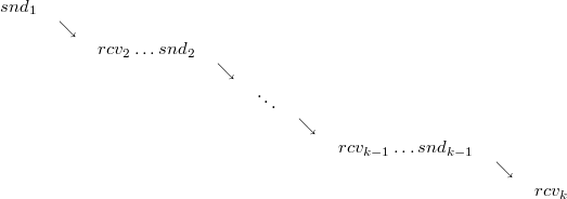
for  , such that
  is either equal to
  or is executed after
  by the same processor that executes
  ;
;  is either equal to
  or is executed before
  by the same processor that executes
  ;
;  is executed before
  by the same processor,
  ; and
; and  sends a message that is received by
  ,
,  . Note that no instruction happens before itself. We write
  when
when  happens before
  . We omit the reference to the execution for which the relation is defined, because it will be clear from the context which execution we mean. We say that two instructions
  and
and  are concurrent when neither
  nor
nor  . The question stands how processors can determine if one instruction happens before another in a given execution according to our definition. This question can be answered through a generalisation of the
 Logical-Clock algorithm presented earlier. This generalisation is called vector clocks.
The Vector-Clocks algorithm allows processors to relate instructions, and this relation is exactly the happens before relation. Each processor  maintains a vector
  of
of  integers. The
  -th coordinate of the vector is denoted by
  . The vector is initialised to the zero vector
  . A vector is modified each time processor executes an instruction, in a way similar to the way counter was modified in the
 Logical-Clock algorithm. Specifically, when a processor  executes any instruction other than sending or receiving a message, the coordinate
  gets incremented by one, and other coordinates remain intact. When a processor sends a message, it increments
  by one, and attaches the resulting vector
  to the message. When a processor
  receives a message, then the processor retrieves the vector
  attached to the message, calculates coordinate-wise maximum of the current vector
  and the vector
  , except for coordinate
  that gets incremented by one, and assigns the result to the variable
  .
.
FOR ALL

We label each instruction  executed by processor
  with the value of the vector
  right after the instruction has been executed. The label is denoted by
  and is called vector timestamp of instruction
  . Intuitively,
  represents the knowledge of processor
  about how many instructions each processor has executed at the moment when
  has executed instruction
  . This knowledge may be obsolete.
Vector timestamps can be used to order instructions that have been executed. Specifically, given two instructions  and
and  , and their vector timestamps
  and
and  , we write that
  when the vector
  is majorised by the vector
  i.e., for all
  , the coordinate
  is at most the corresponding coordinate
  . We write
  when
when  but
but  .
.
The next theorem explains that the Vector-Clocks algorithm indeed implements the happens before relation, because we can decide if two instructions happen or not before each other, just by comparing the vector timestamps of the instructions.
Theorem 13.23 For any execution and any two instructions  and
and  ,
,  if and only if
  .
.
Proof. We first show the forward implication. Suppose that  . Hence
  and
and  are two different instructions. If the two instructions are executed on the same processor, then
  must be executed before
  . Only finite number of instructions have been executed by the time
  has been executed. The
 Vector-Clock algorithm increases a coordinate by one as it calculates vector timestamps of instructions from  until
until  inclusive, and no coordinate is ever decreased. Thus
  . If
. If  and
and  were executed on different processors, then by the definition of happens before relation, there must be a finite chain of instructions and messages leading from
  to
to  . But then by the
 Vector-Clock algorithm, the value of a coordinate of vector timestamp gets increased at each move, as we move along the chain, and so again  .
.
Now we show the reverse implication. Suppose that it is not the case that  . We consider a few subcases always concluding that it is not that case that
  . First, it could be the case that
  and
and  are the same instruction. But then obviously vector clocks assigned to
  and
and  are the same, and so it cannot be the case that
  . Let us, therefore, assume that
  and
and  are different instructions. If they are executed by the same processor, then
  cannot be executed before
  , and so
  is executed after
  . Thus, by monotonicity of vector timestamps,
  , and so it is not the case that
  . The final subcase is when
  and
and  are executed by two distinct processors
  and
and  . Let us focus on the component
  of vector clock
  of processor
  right after
  was executed. Let its value be
  . Recall that other processors can only increase the value of their components
  by adopting the value sent by other processors. Hence, in order for the value of component
  of processor
  to be
to be  or more at the moment
  is executed, there must be a chain of instructions and messages that passes a value at least
  , originating at processor
  . This chain starts at
  or at an instruction executed by
  subsequent to
  . But the existence of such chain would imply that
  happens before
  , which we assumed was not the case. So the component
  of vector clock
  is strictly smaller than the component
  of vector clock
  . Thus it cannot be the case that
  .
.
This theorem tells us that we can decide if two distinct instructions  and
and  are concurrent, by checking that it is not the case that
  nor is it the case that
  .
.
The happens before relation can be used to compute a global state of distributed system, such that this state is in some sense consistent. Shortly, we will formally define the notion of consistency. Each processor executes instructions. A cut  is defined as a vector
  of non-negative integers. Intuitively, the vector
  denotes the states of processors. Formally,
  denotes the number of instructions that processor
  has executed. Not all cuts correspond to collections of states of distributed processors that could be considered natural or consistent. For example, if a processor
  has received a message from
  and we record the state of
  in the cut by making
  appropriately large, but make
  so small that the cut contains the state of the sender before the moment when the message was sent, then we could say that such cut is not natural—there are instructions recorded in the cut that are causally affected by instructions that are not recorded in the cut. Such cuts we consider not consistent and so undesirable. Formally, a cut
  is inconsistent when there are processors
  and
and  such that the instruction number
  of processor
  is causally affected by an instruction subsequent to instruction number
  of processor
  . So in an inconsistent cut there is a message that “crosses” the cut in a backward direction. Any cut that is not inconsistent is called a consistent cut.
The Consistent-Cut algorithm uses vector timestamps to find a consistent cut. We assume that each processor is given the same cut  as an input. Then processors must determine a consistent cut
  that is majorised by
  . Each processor
  has an infinite table
  of vectors. Processor executes instructions, and stores vector timestamps in consecutive entries of the table. Specifically, entry
  of the table is the vector timestamp
  of the
  -th instruction executed by the processor; we define
  to be the zero vector. Processor
  begins calculating a cut right after the moment when the processor has executed instruction number
  . The processor determines the largest number
  that is at most
  , such that the vector
  is majorised by
  . The vector
  that processors collectively find turns out to be a consistent cut.
Theorem 13.24 For any cut  , the cut
  computed by the
 Consistent-Cut algorithm is a consistent cut majorised by  .
.
Proof. First observe that there is no need to consider entries of  further than
  . Each of these entries is not majorised by
  , because the
  -th coordinate of any of these vectors is strictly larger than
  . So we can indeed focus on searching among the first
  entries of
  . Let
. Let  be the largest entry such that the vector
  is majorised by the vector
  . We know that such vector exists, because
  is a zero vector, and such vector is majorised by any cut
  .
.
We argue that  is a consistent cut by way of contradiction. Suppose that the vector
  is an inconsistent cut. Then, by definition, there are processors
  and
and  such that there is an instruction
  of processor
  subsequent to instruction number
  , such that
  happens before instruction number
  of processor
  . Recall that
  is the furthest entry of
  majorised by
  . So entry
  is not majorised by
  , and since all subsequent entries, including the one for instruction
  , can have only larger coordinates, the entries are not majorised by
  either. But,
  happens before instruction number
  , so entry
  can only have larger coordinates than respective coordinates of the entry corresponding to
  , and so
  cannot be majorised by
  either. This contradicts the assumption that
  is majorised by
  . Therefore,
  must be a consistent cut.
There is a trivial algorithm for finding a consistent cut. The algorithm picks  . However, the
 Consistent-Cut algorithm is better in the sense that the consistent cut found is maximal. That this is indeed true, is left as an exercise.
There is an alternative way to find a consistent cut. The Consistent Cut algorithm requires that we attach vector timestamps to messages and remember vector timestamps for all instructions executed so far by the algorithm  which consistent cut we want to compute. This may be too costly. The algorithm called
 Distributed-Snapshot avoids this cost. In the algorithm, a processor initiates the calculation of consistent cut by flooding the network with a special message that acts like a sword that cuts the execution of algorithm  consistently. In order to prove that the cut is indeed consistent, we require that messages are received by the recipient in the order they were sent by the sender. Such ordering can be implemented using sequence number.
In the Distributed-Snapshot algorithm, each processor  has a variable called counter that counts the number of instructions of algorithm
  executed by the processor so far. In addition the processor has a variable
  that will store the
  -th coordinate of the cut. This variable is initialised to
  . Since the variables counter only count the instructions of algorithm
  , the instructions of
 Distributed-Snapshot algorithm do not affect the counter variables. In some sense the snapshot algorithm runs in the “background”. Suppose that there is exactly one processor that can decide to take a snapshot of the distributed system. Upon deciding, the processor “floods” the network with a special message <Snapshot>. Specifically, the processor sends the message to all its neighbours and assigns counter to  . Whenever a processor
  receives the message and the variable
  is still
  , then the processor sends <Snapshot> message to all its neighbours and assigns current to
  . The sending of <Snapshot> messages and assignment are done by the processor without executing any instruction of
  (we can think of
 Distributed-Snapshot algorithm as an “interrupt”). The algorithm calculates a consistent cut.
Theorem 13.25 Let for any processors  and
and  , the messages sent from
  to
to  be received in the order they are sent. The
 Distributed-Snapshot algorithm eventually finds a consistent cut  . The algorithm sends
  messages, where
  is the number of edges in the graph.
Proof. The fact that each variable  is eventually different from
  follows from our model, because we assumed that instructions are eventually executed and messages are eventually received, so the <Snapshot> messages will eventually reach all nodes.
Suppose that  is not a consistent cut. Then there is a processor
  such that instruction number
  or later sends a message <
  > other than <Snapshot>, and the message is received on or before a processor
  executes instruction number
  . So the message <
  > must have been sent after the message <Snapshot> was sent from
  to
to  . But messages are received in the order they are sent, so
  processes <Snapshot> before it processes <
  >. But then message <
  > arrives after snapshot was taken at
  . This is a desired contradiction.
Exercises
13.5-1 Show that logical time preserves the happens before ( ) relation. That is, show that if for events
  and
and  it is the case that
  , then
  , where
  is the logical time of an event.
13.5-2 Show that any vector clock that captures concurrency between  processors must have at least
  coordinates.
13.5-3 Show that the vector  calculated by the algorithm
 Consistent-Cut is in fact a maximal consistent cut majorised by  . That is that there is no
  that majorises
  and is different from
  , such that
  is majorised by
  .
.
Among the fundamental problems in distributed systems where processors communicate by message passing are the tasks of spreading and gathering information. Many distributed algorithms for communication networks can be constructed using building blocks that implement various broadcast and multicast services. In this section we present some basic communication services in the message-passing model. Such services typically need to satisfy some quality of service requirements dealing with ordering of messages and reliability. We first focus on broadcast services, then we discuss more general multicast services.
In the broadcast problem, a selected processor  , called a source or a sender, has the message
  , which must be delivered to all processors in the system (including the source). The interface of the broadcast service is specified as follows:
-
bc-send
 : an event of processor
  that sends a message
  to all processors.
 -
bc-recv
 : an event of processor
  that receives a message
  sent by processor
  .
.
In above definitions qos denotes the quality of service provided by the system. We consider two kinds of quality service:
-
Ordering: how the order of received messages depends on the order of messages sent by the source?
-
Reliability: how the set of received messages depends on the failures in the system?
The basic model of a message-passing distributed system normally does not guarantee any ordering or reliability of messaging operations. In the basic model we only assume that each pair of processors is connected by a link, and message delivery is independent on each link — the order of received messages may not be related to the order of the sent messages, and messages may be lost in the case of crashes of senders or receivers.
We present some of the most useful requirements for ordering and reliability of broadcast services. The main question we address is how to implement a stronger service on top of the weaker service, starting with the basic system model.
Applying the definition of happens before to messages, we say that message  happens before message
  if either
  and
and  are sent by the same processor and
  is sent before
  , or the bc-recv event for
  happens before the bc-send event for
  .
.
We identify four common broadcast services with respect to the message ordering properties:
-
Basic Broadcast: no order of messages is guaranteed.
-
Single-Source FIFO (first-in-first-out): messages sent by one processor are received by each processor in the same order as sent; more precisely, for all processors
 and messages
  , if processor
  sends
sends  before it sends
  then processor
  does not receive message
  before message
  .
. -
Causal Order: messages are received in the same order as they happen; more precisely, for all messages
 and every processor
  , if
, if  happens before
  then
then  does not receive
  before
  .
. -
Total Order: the same order of received messages is preserved in each processor; more precisely, for all processors
 and messages
  , if processor
  receives
  before it receives
  then processor
  does not receive message
  before message
  .
.
It is easy to see that Causal Order implies Single-Source FIFO requirements (since the relation “happens before” for messages includes the order of messages sent by one processor), and each of the given services trivially implies Basic Broadcast. There are no additional relations between these four services. For example, there are executions that satisfy Single-Source FIFO property, but not Causal Order. Consider two processors  and
and  . In the first event
  broadcasts message
  , next processor
  receives
  , and then
  broadcasts message
  . It follows that
  happens before
  . But if processor
  receives
  before
  , which may happen, then this execution violates Causal Order. Note that trivially Single-Source FIFO requirement is preserved, since each processor broadcasts only one message.
We denote by  the Basic Broadcast service, by ssf the Single-Source FIFO, by
  the Causal Order and by
  the Total Order service.
In the model without failures we would like to guarantee the following properties of broadcast services:
-
Integrity: each message
 received in event bc-recv has been sent in some bc-send event.
 -
No-Duplicates: each processor receives a message not more than once.
-
Liveness: each message sent is received by all processors.
In the model with failures we define the notion of reliable broadcast service, which satisfies Integrity, No-Duplicates and two kinds of Liveness properties:
-
Nonfaulty Liveness: each message
 sent by non-faulty processor
  must be received by every non-faulty processor.
 -
Faulty Liveness: each message sent by a faulty processor is either received by all non-faulty processors or by none of them.
We denote by rbb the Reliable Basic Broadcast service, by rssf the Reliable Single-Source FIFO, by  the Reliable Causal Order, and by rto the Reliable Total Order service.
We now describe implementations of algorithms for various broadcast services.
The bb service is implemented as follows. If event  occurs then processor
  sends message
  via every link from
  to
to  , where
  . If a message
  comes to processor
  then it enables event
  .
.
To provide reliability we do the following. We build the reliable broadcast on the top of basic broadcast service. When  occurs, processor
  enables event
  . If event
  occurs and message-coordinate
  appears for the first time then processor
  first enables event
  (to inform other non-faulty processors about message
  in case when processor
  is faulty), and next enables event
  .
.
We prove that the above algorithm provides reliability for the basic broadcast service. First observe that Integrity and No-Duplicates properties follow directly from the fact that each processor  enables
  only if message-coordinate
  is received for the first time. Nonfaulty liveness is preserved since links between non-faulty processors enables events
  correctly. Faulty Liveness is guaranteed by the fact that if there is a non-faulty processor
  which receives message
  from the faulty source
  , then before enabling
  processor
  sends message
  using
using  event. Since
  is non-faulty, each non-faulty processor
  gets message
  in some
  event, and then accepts it (enabling event
  ) during the first such event.
Each processor  has its own counter (timestamp), initialised to
  . If event
  occurs then processor
  sends message
  with its current timestamp attached, using
  . If an event
  occurs then processor
  enables event
  just after events
  have been enabled, where
  are the messages such that events
  have been enabled.
Note that if we use reliable Basic Broadcast instead of Basic Broadcast as the background service, the above implementation of Single-Source FIFO becomes Reliable Single-Source FIFO service. We leave the proof to the reader as an exercise.
We present an ordered broadcast algorithm which works in the asynchronous message-passing system providing single-source FIFO broadcast service. It uses the idea of timestamps, but in more advanced way than in the implementation of ssf. We denote by cto the service satisfying causal and total orders requirements.
Each processor  maintains in a local array
  its own increasing counter (timestamp), and the estimated values of timestamps of other processors. Timestamps are used to mark messages before sending—if
  is going to broadcast a message, it increases its timestamp and uses it to tag this message (lines 11-13). During the execution processor
  estimates values of timestamps of other processors in the local vector
  —if processor
  receives a message from processor
  with a tag
  (timestamp of
  ), it puts
  into
into  (lines 23–32). Processor
  sets its current timestamp to be the maximum of the estimated timestamps in the vector
  plus one (lines 24–26). After updating the timestamp processor sends an update message. Processor accepts a message
  with associated timestamp
  from processor
  if pair
  is the smallest among other received messages (line 42), and each processor has at least as large a timestamp as known by processor
  (line 43). The details are given in the code below.
Ordered-Broadcast
Code for any processor,
<01>
INITIALISATION</01> <02>for every
</02> 11
IFoccurs 12
THEN13
ENABLE21
IFoccurs 22
THENADDtripleto pending 23
24
IF25
THEN26
ENABLE31
IFoccurs 32
THEN41
IF42is the pending triple with the smallest
and
for every
43
THENENABLE44
REMOVEtriplefrom pending
Ordered-Broadcast satisfies the causal order requirement. We leave the proof to the reader as an exercise (in the latter part we show how to achieve stronger reliable causal order service and provide the proof for that stronger case).
Theorem 13.26 Ordered-Broadcast satisfies the total order requirement.
Proof. Integrity follows from the fact that each processor can enable event  only if the triple
  is pending (lines 41–45), which may happen after receiving a message
  from processor
  (lines 21–22). No-Duplicates property is guaranteed by the fact that there is at most one pending triple containing message
  sent by processor
  (lines 13 and 21–22).
Liveness follows from the fact that each pending triple satisfies conditions in lines 42–43 in some moment of the execution. The proof of this fact is by induction on the events in the execution — suppose to the contrary that  is the triple with smallest
  which does not satisfy conditions in lines 42–43 at any moment of the execution. It follows that there is a moment from which triple
  has smallest
  coordinates among pending triples in processor
  . Hence, starting from this moment, it must violate condition in line 43 for some
  . Note that
  , by updating rules in lines 23–25. It follows that processor
  never receives a message from
  with timestamp greater than
  , which by updating rules in lines 24–26 means that processor
  never receives a message
  from
from  , which contradicts the liveness property of
  broadcast service.
To prove Total Order property it is sufficient to prove that for every processor  and messages
  sent by processors
  with timestamps
  respectively, each of the triples
  ,
,  are accepted according to the lexicographic order of
  . There are two cases.
Case 1. Both triples are pending in processor  at some moment of the execution. Then condition in line 42 guarantees acceptance in order of
  .
.
Case 2. Triple  (without loss of generality) is accepted by processor
  before triple
  is pending. If
  then still the acceptance is according to the order of
  . Otherwise
  , and by condition in line 43 we get in particular that
  , and consequently
  . This can not happen because of the ssf requirement and the assumption that processor
  has not yet received message
  from
from  via the
  broadcast service.
Now we address reliable versions of Causal Order and Total Order services. A Reliable Causal Order requirements can be implemented on the top of Reliable Basic Broadcast service in asynchronous message-passing system with processor crashes using the following algorithm. It uses the same data structures as previous Ordered-Bbroadcast. The main difference between reliable Causally-Ordered-Broadcast and Ordered-Broadcast are as follows: instead of using integer timestamps processors use vector timestamps  , and they do not estimate timestamps of other processors, only compare in lexicographic order their own (vector) timestamps with received ones. The intuition behind vector timestamp of processor
  is that it stores information how many messages have been sent by
  and how many have been accepted by
  from every
  , where
  .
.
In the course of the algorithm processor  increases corresponding position
  in its vector timestamp
  before sending a new message (line 12), and increases
  th position of its vector timestamp after accepting new message from processor
  (line 38). After receiving a new message from processor
  together with its vector timestamp
  , processor
  adds triple
  to pending and accepts this triple if it is first not accepted message received from processor
  (condition in line 33) and the number of accepted messages (from each processor
  ) by processor
  was not bigger in the moment of sending
  than it is now in processor
  (condition in line 34). Detailed code of the algorithm follows.
Reliable-Causally-Ordered-Broadcast
Code for any processor,
<01>
INITIALISATION</01> <02>for every
</02> <03> pending list is empty</03> 11
IFoccurs 12
THEN13
ENABLE21
IFoccurs 22
THENADDtripleto pending 31
IFis the pending triple, and 32
, and 33
for every
34
THENENABLE35
REMOVEtriplefrom pending 36
We argue that the algorithm Reliable-Causally-Ordered-Broadcast provides Reliable Causal Order broadcast service on the top of the system equipped with the Reliable Basic Broadcast service. Integrity and No-Duplicate properties are guaranteed by rbb broadcast service and facts that each message is added to pending at most once and non-received message is never added to pending. Nonfaulty and Faulty Liveness can be proved by one induction on the execution, using facts that non-faulty processors have received all messages sent, which guarantees that conditions in lines 33–34 are eventually satisfied. Causal Order requirement holds since if message  happens before message
  then each processor
  accepts messages
  according to the lexicographic order of
  , and these vector-arrays are comparable in this case. Details are left to the reader.
Note that Reliable Total Order broadcast service can not be implemented in the general asynchronous setting with processor crashes, since it would solve consensus in this model — first accepted message would determine the agreement value (against the fact that consensus is not solvable in the general model).
Multicast services are similar to the broadcast services, except each multicast message is destined for a specified subset of all processors.In the multicast service we provide two types of events, where qos denotes a quality of service required:
-
 : an event of processor
  which sends a message
  together with its id to all processors in a destination set
  .
. -
 : an event of processor
  which receives a message
  sent by processor
  .
.
Note that the event mc-recv is similar to bc-recv.
As in case of a broadcast service, we would like to provide useful ordering and reliable properties of the multicast services. We can adapt ordering requirements from the broadcast services. Basic Multicast does not require any ordering properties. Single-Source FIFO requires that if one processor multicasts messages (possibly to different destination sets), then the messages received in each processors (if any) must be received in the same order as sent by the source. Definition of Causal Order remains the same. Instead of Total Order, which is difficult to achieve since destination sets may be different, we define another ordering property:
-
Sub-Total Order: orders of received messages in all processors may be extended to the total order of messages; more precisely, for any messages
 and processors
  , if
, if  and
and  receives both messages
  then they are received in the same order by
  and
and  .
.
The reliability conditions for multicast are somewhat different from the conditions for reliable broadcast.
-
Integrity: each message
 received in event
  was sent in some mc-send event with destination set containing processor
  .
. -
No Duplicates: each processor receives a message not more than once.
-
Nonfaulty Liveness: each message
 sent by non-faulty processor
  must be received in every non-faulty processor in the destination set.
 -
Faulty Liveness: each message sent by a faulty processor is either received by all non-faulty processors in the destination set or by none of them.
One way of implementing ordered and reliable multicast services is to use the corresponding broadcast services (for Sub-Total Order the corresponding broadcast requirement is Total Order). More precisely, if event  occurs processor
  enables event
  . When an event
  occurs, processor
  enables event
  if
if  , otherwise it ignores this event. The proof that such method provides required multicast quality of service is left as an exercise.
Reliable multicast services can be used as building blocks in constructing algorithms for more advanced communication problems. In this section we illustrate this method for the problem of collecting rumors by synchronous processors prone to crashes. (Since we consider only fair executions, we assume that at least one processor remains operational to the end of the computation).
The classic problem of collecting rumors, or gossip, is defined as follows:
At the beginning, each processor has its distinct piece of information, called a rumor, the goal is to make every processor know all the rumors.
However in the model with processor crashes we need to re-define the gossip problem to respect crash failures of processors. Both Integrity and No-Duplicates properties are the same as in the reliable broadcast service, the only difference (which follows from the specification of the gossip problem) is in Liveness requirements:
-
Non-faulty Liveness: the rumor of every non-faulty processor must be known by each non-faulty processor.
-
Faulty Liveness: if processor
 has crashed during execution then each non-faulty processor either knows the rumor of
  or knows that
  is crashed.
The efficiency of gossip algorithms is measured in terms of time and message complexity. Time complexity measures number of (synchronous) steps from the beginning to the termination. Message complexity measures the total number of point-to-point messages sent (more precisely, if a processor sends a message to three other processors in one synchronous step, it contributes three to the message complexity).
The following simple algorithm completes gossip in just one synchronous step: each processor broadcasts its rumor to all processors. The algorithm is correct, because each message received contains a rumor, and a message not received means the failure of its sender. A drawback of such a solution is that a quadratic number of messages could be sent, which is quite inefficient.
We would like to perform gossip not only quickly, but also with fewer point-to-point messages. There is a natural trade-off between time and communication. Note that in the system without processor crashes such a trade-off may be achieved, e.g., sending messages over the (almost) complete binary tree, and then time complexity is  , while the message complexity is
  . Hence by slightly increasing time complexity we may achieve almost linear improvement in message complexity. However, if the underlying communication network is prone to failures of components, then irregular failure patterns disturb a flow of information and make gossiping last longer. The question we address in this section is what is the best trade-off between time and message complexity in the model with processor crashes?
In this part we describe the family of gossip algorithms, among which we can find some efficient ones. They are all based on the same generic code, and their efficiency depends on the quality of two data structures put in the generic algorithm. Our goal is to prove that we may find some of those data structures that obtained algorithm is always correct, and efficient if the number of crashes in the execution is at most  , where
  is a parameter.
We start with description of these structures: communication graph and communication schedules.
A graph  consists of a set
  of vertices and a set
  of edges. Graphs in this paper are always simple, which means that edges are pairs of vertices, with no direction associated with them. Graphs are used to describe communication patterns. The set
  of vertices of a graph consists of the processors of the underlying distributed system. Edges in
  determine the pairs of processors that communicate directly by exchanging messages, but this does not necessarily mean an existence of a physical link between them. We abstract form the communication mechanism: messages that are exchanged between two vertices connected by an edge in
  may need to be routed and traverse a possibly long path in the underlying physical communication network. Graph topologies we use, for a given number
  of processors, vary depending on an upper bound
  on the number of crashes we would like to tolerate in an execution. A graph that matters, at a given point in an execution, is the one induced by the processors that have not crashed till this step of the execution.
To obtain an efficient gossip algorithm, communication graphs should satisfy some suitable properties, for example the following property  :
:
Definition 13.27 Let  be a pair of positive integers. Graph
  is said to satisfy property
  , if
, if  has
has  vertices, and if, for each subgraph
  of size at least
  , there is a subgraph
  of
of  , such that the following hold:
1: 
2: 
3: The diameter of  is at most
4: If  , then
In the above definition, clause (1.) requires the existence of subgraphs  whose vertices has the potential of (informally) inheriting the properties of the vertices of
  , clause (2.) requires the subgraphs to be sufficiently large, linear in size, clause (3.) requires the existence of paths in the subgraphs that can be used for communication of at most logarithmic length, and clause (4.) imposes monotonicity on the required subgraphs. Observe that graph
  is connected, even if
  is not, since its diameter is finite. The following result shows that graphs satisfying property
  can be constructed, and that their degree is not too large.
Theorem 13.28 For each  , there exists a graph
  satisfying property
  . The maximum degree
  of graph
  is
is  .
.
A local permutation is a permutation of all the integers in the range  . We assume that prior the computation there is given set
  of
of  local permutations. Each processor
  has such a permutation
  from
from  . For simplicity we assume that
  . Local permutation is used to collect rumor in systematic way according to the order given by this permutation, while communication graphs are rather used to exchange already collected rumors within large and compact non-faulty graph component.
We start with specifying a goal that gossiping algorithms need to achieve. We say that processor  has heard about processor
  if either
  knows the original input rumor of
  or
or  knows that
  has already failed. We may reformulate correctness of a gossiping algorithm in terms of hearing about other processors: algorithm is correct if Integrity and No-Duplicates properties are satisfied and if each processor has hard about any other processor by the termination of the algorithm.
The code of a gossiping algorithm includes objects that depend on the number  of processors in the system, and also on the bound
  on the number of failures which are “efficiently tolerated” (if the number of failures is at most
  then message complexity of design algorithm is small). The additional parameter is a termination threshold
  which influences time complexity of the specific implementation of the generic gossip scheme. Our goal is to construct the generic gossip algorithm which is correct for any additional parameters
  and any communication graph and set of schedules, while efficient for some values
  and structures
  and
and  .
.
Each processor starts gossiping as a collector. Collectors seek actively information about rumors of the other processors, by sending direct inquiries to some of them. A collector becomes a disseminator after it has heard about all the processors. Processors with this status disseminate their knowledge by sending local views to selected other processors.
Local views. Each processor  starts with knowing only its ID and its input information
  . To store incoming data, processor
  maintains the following arrays:
 , ,  and and  , , |
each of size  . All these arrays are initialised to store the value
 nil. For an array  of processor
  , we denote its
  th entry by
  - intuitively this entry contains some information about processor
  . The array
 Rumor is used to store all the rumors that a processor knows. At the start, processor  sets
sets  to its own input
  . Each time processor
  learns some
  , it immediately sets
  to this value. The array
 Active is used to store a set of all the processors that the owner of the array knows as crashed. Once processor  learns that some processor
  has failed, it immediately sets
  to failed. Notice that processor
  has heard about processor
  , if one among the values
  and
and  is not equal to
 NIL.
The purpose of using the array Pending is to facilitate dissemination. Each time processor  learns that some other processor
  is fully informed, that is, it is either a disseminator itself or has been notified by a disseminator, then it marks this information in
  . Processor
  uses the array
  to send dissemination messages in a systematic way, by scanning
  to find those processors that possibly still have not heard about some processor.
The following is a useful terminology about the current contents of the arrays Active and Pending. Processor  is said to be active according to
  , if
, if  has not yet received any information implying that
  crashed, which is the same as having
 nil in  . Processor
  is said to need to be notified by
  if it is active according to
  and
and  is equal to
 nil.
Phases. An execution of a gossiping algorithm starts with the processors initialising all the local objects. Processor  initialises its list
  with
with nil at all the locations, except for the  th one, which is set equal to
  . The remaining part of execution is structured as a loop, in which phases are iterated. Each phase consists of three parts: receiving messages, local computation, and multicasting messages. Phases are of two kinds: regular phase and ending phase. During regular phases processor: receives messages, updates local knowledge, checks its status, sends its knowledge to neighbours in communication graphs as well as inquiries about rumors and replies about its own rumor. During ending phases processor: receives messages, sends inquiries to all processors from which it has not heard yet, and replies about its own rumor. The regular phases are performed
  times; the number
  is a termination threshold. After this, the ending phase is performed four times. This defines a generic gossiping algorithm.
Generic-Gossip
Code for any processor,
<01>
INITIALISATION</01> <02> processorbecomes a collector</02> <03> initialisation of arrays
,
and
</03> 11
REPEATtimes 12
PERFORMregular phase 20REPEATtimes 21
PERFORMending phase
Now we describe communication and kinds of messages used in regular and ending phases.
Graph and range messages used during regular phases. A processor  may send a message to its neighbour in the graph
  , provided that it is is still active according to
  . Such a message is called a graph one. Sending these messages only is not sufficient to complete gossiping, because the communication graph may become disconnected as a result of node crashes. Hence other messages are also sent, to cover all the processors in a systematic way. In this kind of communication processor
  considers the processors as ordered by its local permutation
  , that is, in the order
  . Some of additional messages sent in this process are called range ones.
During regular phase processors send the following kind of range messages: inquiring, reply and notifying messages. A collector  sends an inquiring message to the first processor about which
  has not heard yet. Each recipient of such a message sends back a range message that is called a reply one.
Disseminators send range messages also to subsets of processors. Such messages are called notifying ones. The target processor selected by disseminator  is the first one that still needs to be notified by
  . Notifying messages need not to be replied to: a sender already knows the rumors of all the processors, that are active according to it, and the purpose of the message is to disseminate this knowledge.
Regular-Phase
Code for any processor,
<01>
RECEIVEmessages</01> 11PERFORMlocal computation 12UPDATEthe local arrays 13IFis a collector, that has already heard about all the processors 14
THENbecomes a disseminator 15
COMPUTEset of destination processors:FOReach processor16
IFis active according to
and
is a neighbour of
in graph
17
THENaddto destination set for a graph message 18
IFis a collector and
is the first processor about which
has not heard yet 19
THENsend an inquiring message to20
IFis a disseminator and
is the first processor that needs to be notified by
21
THENsend a notifying message to22
IFis a collector, from which an inquiring message was received in the receiving step of this phase 23
THENsend a reply message to30
SENDgraph/inquiring/notifying/reply messages to corresponding destination sets
Last-resort messages used during ending phases. Messages sent during the ending phases are called last-resort ones. These messages are categorised into inquiring, replying, and notifying, similarly as the corresponding range ones, which is because they serve a similar purpose. Collectors that have not heard about some processors yet send direct inquiries to all of these processors simultaneously. Such messages are called inquiring ones. They are replied to by the non-faulty recipients in the next step, by way of sending reply messages. This phase converts all the collectors into disseminators. In the next phase, each disseminator sends a message to all the processors that need to be notified by it. Such messages are called notifying ones.
The number of graph messages, sent by a processor at a step of the regular phase, is at most as large as the maximum node degree in the communication graph. The number of range messages, sent by a processor in a step of the regular phase, is at most as large as the number of inquiries received plus a constant - hence the global number of point-to-point range messages sent by all processors during regular phases may be accounted as a constant times the number of inquiries sent (which is one per processor per phase). In contrast to that, there is no a priori upper bound on the number of messages sent during the ending phase. By choosing the termination threshold  to be large enough, one may control how many rumors still needs to be collected during the ending phases.
Updating local view. A message sent by a processor carries its current local knowledge. More precisely, a message sent by processor  brings the following: the ID
  , the arrays
  ,
,  , and
, and  , and a label to notify the recipient about the character of the message. A label is selected from the following: graph_message, inquiry_from_collector, notification_from_disseminator, this_is_a_reply, their meaning is self-explanatory. A processor
  scans a newly received message from some processor
  to learn about rumors, failures, and the current status of other processors. It copies each rumor from the received copy of
  into
into  , unless it is already there. It sets
  to failed, if this value is at
  . It sets
  to done, if this value is at
  . It sets
  to done, if
  is a disseminator and the received message is a range one. If
  is itself a disseminator, then it sets
  to done immediately after sending a range message to
  . If a processor
  expects a message to come from processor
  , for instance a graph one from a neighbour in the communication graph, or a reply one, and the message does not arrive, then
  knows that processor
  has failed, and it immediately sets
  to failed.
Ending-Phase
Code for any processor,
<01>
RECEIVEmessages</01> 11PERFORMlocal computation 12UPDATEthe local arrays 13IFis a collector, that has already heard about all the processors 14
THENbecomes a disseminator 15
COMPUTEset of destination processors:FOReach processor16
IFis a collector and it has not heard about
yet 17
THENsend an inquiring message to18
IFis a disseminator and
needs to be notified by
19
THENsend a notifying message to20
IFan inquiring message was received fromin the receiving step of this phase 21
THENsend a reply message to30
SENDinquiring/notifying/reply messages to corresponding destination sets
Correctness. Ending phases guarantee correctness, as is stated in the next fact.
Lemma 13.29 Generic-Gossip is correct for every communication graph  and set of schedules
  .
.
Proof. Integrity and No-Duplicates properties follow directly from the code and the multicast service in synchronous message-passing system. It remains to prove that each processor has heard about all processors. Consider the step just before the first ending phases. If a processor  has not heard about some other processor
  yet, then it sends a last-resort message to
  in the first ending phase. It is replied to in the second ending phase, unless processor
  has crashed already. In any case, in the third ending phase, processor
  either learns the input rumor of
  or it gets to know that
  has failed. The fourth ending phase provides an opportunity to receive notifying messages, by all the processors that such messages were sent to by
  .
.
The choice of communication graph  , set of schedules
  and termination threshold
  influences however time and message complexities of the specific implementation of Generic Gossip Algorithm. First consider the case when
  is a communication graph satisfying property
  from Definition 13.27,
  contains
  random permutations, and
  for sufficiently large positive constant
  . Using Theorem 13.28 we get the following result.
Theorem 13.30 For every  and
and  , for some constant
  , there is a graph
  such that the implementation of the generic gossip scheme with
  as a communication graph and a set
  of random permutations completes gossip in expected time
  and with expected message complexity
  , if the number of crashes is at most
  .
.
Consider a small modification of Generic Gossip scheme: during regular phase every processor  sends an inquiring message to the first
  (instead of one) processors according to permutation
  , where
  is a maximum degree of used communication graph
  . Note that it does not influence the asymptotic message complexity, since besides inquiring messages in every regular phase each processor
  sends
sends  graph messages.
Theorem 13.31 For every  there are parameters
  and
and  and there is a graph
  such that the implementation of the modified Generic Gossip scheme with
  as a communication graph and a set
  of random permutations completes gossip in expected time
  and with expected message complexity
  , for any number of crashes.
Since in the above theorem set  is selected prior the computation, we obtain the following existential deterministic result.
Theorem 13.32 For every  there are parameters
  and
and  and there are graph
  and set of schedules
  such that the implementation of the modified Generic Gossip scheme with
  as a communication graph and schedules
  completes gossip in time
  and with message complexity
  , for any number of crashes.
Exercises
13.7-1 Design executions showing that there is no relation between Causal Order and Total Order and between Single-Source FIFO and Total Order broadcast services. For simplicity consider two processors and two messages sent.
13.7-2 Does broadcast service satisfying Single-Source FIFO and Causal Order requirements satisfy a Total Order property? Does broadcast service satisfying Single-Source FIFO and Total Order requirements satisfy a Causal Order property? If yes provide a proof, if not show a counterexample.
13.7-3 Show that using reliable Basic Broadcast instead of Basic Broadcast in the implementation of Single-Source FIFO service, then we obtain reliable Single-Source FIFO broadcast.
13.7-4 Prove that the Ordered Broadcast algorithm implements Causal Order service on a top of Single-Source FIFO one.
13.7-5 What is the total number of point-to-point messages sent in the algorithm Ordered-Broadcast in case of  broadcasts?
13.7-6 Estimate the total number of point-to-point messages sent during the execution of Reliable-Causally-Ordered-Broadcast, if it performs  broadcast and there are
  processor crashes during the execution.
13.7-7 Show an execution of the algorithm Reliable-Causally-Ordered-Broadcast which violates Total Order requirement.
13.7-8 Write a code of the implementation of reliable Sub-Total Order multicast service.
13.7-9 Show that the described method of implementing multicast services on the top of corresponding broadcast services is correct.
13.7-10 Show that the random graph  - in which each node selects independently at random
  edges from itself to other processors - satisfies property
  from Definition 13.27 and has degree
  with probability at least
  .
.
13.7-11 Leader election problem is as follows: all non-faulty processors must elect one non-faulty processor in the same synchronous step. Show that leader election can not be solved faster than gossip problem in synchronous message-passing system with processors crashes.
We now describe the second main model used to describe distributed systems, the shared memory model. To illustrate algorithmic issues in this model we discuss solutions for the mutual exclusion problem.
The shared memory is modeled in terms of a collection of shared variables, commonly referred to as registers. We assume the system contains  processors,
  , and
, and  registers
  . Each processor is modeled as a state machine. Each register has a type, which specifies:
-
the values it can hold,
-
the operations that can be performed on it,
-
the value (if any) to be returned by each operation, and
-
the new register value resulting from each operation.
Each register can have an initial value.
For example, an integer valued read/write register  can take on all integer values and has operations read(R,v) and write(R,v). The read operation returns the value
  of the last preceding write, leaving
  unchanged. The write(R,v) operation has an integer parameter
  , returns no value and changes
  's value to
  . A configuration is a vector
  , where
  is a state of
  and
and  is a value of register
  . The events are computation steps at the processors where the following happens atomically (indivisibly):
-
 chooses a shared variable to access with a specific operation, based on
  's current state,
 -
the specified operation is performed on the shared variable,
-
 's state changes based on its transition function, based on its current state and the value returned by the shared memory operation performed.
A finite sequence of configurations and events that begins with an initial configuration is called an execution. In the asynchronous shared memory system, an infinite execution is admissible if it has an infinite number of computation steps.
In this problem a group of processors need to access a shared resource that cannot be used simultaneously by more than a single processor. The solution needs to have the following two properties. (1) Mutual exclusion: Each processor needs to execute a code segment called a critical section so that at any given time at most one processor is executing it (i.e., is in the critical section). (2) Deadlock freedom: If one or more processors attempt to enter the critical section, then one of them eventually succeeds as long as no processor stays in the critical section forever. These two properties do not provide any individual guarantees to any processor. A stronger property is (3) No lockout: A processor that wishes to enter the critical section eventually succeeds as long as no processor stays in the critical section forever. Original solutions to this problem relied on special synchronisation support such as semaphores and monitors. We will present some of the distributed solutions using only ordinary shared variables.
We assume the program of a processor is partitioned into the following sections:
-
Entry / Try: the code executed in preparation for entering the critical section.
-
Critical: the code to be protected from concurrent execution.
-
Exit: the code executed when leaving the critical section.
-
Remainder: the rest of the code.
A processor cycles through these sections in the order: remainder, entry, critical and exit. A processor that wants to enter the critical section first executes the entry section. After that, if successful, it enters the critical section. The processor releases the critical section by executing the exit section and returning to the remainder section. We assume that a processor may transition any number of times from the remainder to the entry section. Moreover, variables, both shared and local, accessed in the entry and exit section are not accessed in the critical and remainder section. Finally, no processor stays in the critical section forever. An algorithm for a shared memory system solves the mutual exclusion problem with no deadlock (or no lockout) if the following hold:
-
Mutual Exclusion: In every configuration of every execution at most one processor is in the critical section.
-
No deadlock: In every admissible execution, if some processor is in the entry section in a configuration, then there is a later configuration in which some processor is in the critical section.
-
No lockout: In every admissible execution, if some processor is in the entry section in a configuration, then there is a later configuration in which that same processor is in the critical section.
In the context of mutual exclusion, an execution is admissible if for every processor  ,
,  either takes an infinite number of steps or
  ends in the remainder section. Moreover, no processor is ever stuck in the exit section (unobstructed exit condition).
A single bit suffices to guarantee mutual exclusion with no deadlock if a powerful test&set register is used. A test&set variable  is a binary variable which supports two atomic operations, test&set and reset, defined as follows:
test&set(: memory address) returns binary value:

return (
) reset(
: memory address):

The test&set operation atomically reads and updates the variable. The reset operation is merely a write. There is a simple mutual exclusion algorithm with no deadlock, which uses one test&set register.
Mutual exclusion using one test&set register
Initiallyequals

: 1 wait until
: 2


Assume that the initial value of  is
is  . In the entry section, processor
  repeatedly tests
  until it returns
  . The last such test will assign
  to
to  , causing any following test by other processors to return
  , prohibiting any other processor from entering the critical section. In the exit section
  resets
  to
to  ; another processor waiting in the entry section can now enter the critical section.
Theorem 13.33 The algorithm using one test&set register provides mutual exclusion without deadlock.
If a powerful primitive such as test&set is not available, then mutual exclusion must be implemented using only read/write operations.
Lamport's bakery algorithm for mutual exclusion is an early, classical example of such an algorithm that uses only shared read/write registers. The algorithm guarantees mutual exclusion and no lockout for  processors using
  registers (but the registers may need to store integer values that cannot be bounded ahead of time).
Processors wishing to enter the critical section behave like customers in a bakery. They all get a number and the one with the smallest number in hand is the next one to be “served”. Any processor not standing in line has number  , which is not counted as the smallest number.
The algorithm uses the following shared data structures: Number is an array of  integers, holding in its
  -th entry the current number of processor
  . Choosing is an array of
  boolean values such that
  is true while
  is in the process of obtaining its number. Any processor
  that wants to enter the critical section attempts to choose a number greater than any number of any other processor and writes it into
  . To do so, processors read the array Number and pick the greatest number read
  as their own number. Since however several processors might be reading the array at the same time, symmetry is broken by choosing (
 ,
,  ) as
) as  's ticket. An ordering on tickets is defined using the lexicographical ordering on pairs. After choosing its ticket,
  waits until its ticket is minimal: For all other
  ,
,  waits until
  is not in the process of choosing a number and then compares their tickets. If
  's ticket is smaller,
  waits until
  executes the critical section and leaves it.
Bakery
Code for processor,
. Initially
and
FALSE, for
: 1
TRUE23
FALSE4FOR
TO
DO5WAIT UNTILFALSE6WAIT UNTILor


: 7


We leave the proofs of the following theorems as Exercises 13.8-2 and 13.8-3.
 processors
Lamports Bakery algorithm requires the use of unbounded values. We next present an algorithm that removes this requirement. In this algorithm, first presented by Peterson and Fischer, processors compete pairwise using a two-processor algorithm in a tournament tree arrangement. All pairwise competitions are arranged in a complete binary tree. Each processor is assigned to a specific leaf of the tree. At each level, the winner in a given node is allowed to proceed to the next higher level, where it will compete with the winner moving up from the other child of this node (if such a winner exists). The processor that finally wins the competition at the root node is allowed to enter the critical section.
Let  . Consider a complete binary tree with
  leaves and a total of
  nodes. The nodes of the tree are numbered inductively in the following manner: The root is numbered
  ; the left child of node numbered
  is numbered
  and the right child is numbered
  . Hence the leaves of the tree are numbered
  .
.
With each node  , three binary shared variables are associated:
  , and
, and  . All variables have an initial value of
  . The algorithm is recursive. The code of the algorithm consists of a procedure
 Node  which is executed when a processor accesses node
  , while assuming the role of processor
  . Each node has a critical section. It includes the entry section at all the nodes on the path from the nodes parent to the root, the original critical section and the exit code on all nodes from the root to the nodes parent. To begin, processor
  executes the code of node
  .
.
Tournament-Tree
procedureNode(: integer; side:
) 1
2
WAIT UNTIL(or
) 3
4
IF5
THENIF() 6
THENgoto line 1 7ELSEWAIT UNTIL8
IF9
THEN10
ELSENode() 11
12
end procedure
This algorithm uses bounded values and as the next theorem shows, satisfies the mutual exclusion, no lockout properties:
Theorem 13.36 The tournament tree algorithm guarantees mutual exclusion.
Proof. Consider any execution. We begin at the nodes closest to the leaves of the tree. A processor enters the critical section of this node if it reaches line 9 (it moves up to the next node). Assume we are at a node  that connects to the leaves where
  and
and  start. Assume that two processors are in the critical section at some point. It follows from the code that then
  at this point. Assume, without loss of generality that
  's last write to
  before entering the critical section follows
  's last write to
  before entering the critical section. Note that
  can enter the critical section (of
  ) either through line 5 or line 6. In both cases
  reads
reads  . However
  's read of
  , follows
  's write to
  , which by assumption follows
  's write to
  . Hence
  's read of
  should return
  , a contradiction.
The claim follows by induction on the levels of the tree.
Theorem 13.37 The tournament tree algorithm guarantees no lockout.
Proof. Consider any admissible execution. Assume that some processor  is starved. Hence from some point on
  is forever in the entry section. We now show that
  cannot be stuck forever in the entry section of a node
  . The claim then follows by induction.
Case 1: Suppose  executes line 10 setting
  to 0. Then
  equals
  forever after. Thus
  passes the test in line 2 and skips line 5. Hence
  must be waiting in line 6, waiting for
  to be 0, which never occurs. Thus
  is always executing between lines 3 and 11. But since
  does not stay in the critical section forever, this would mean that
  is stuck in the entry section forever which is impossible since
  will execute line 5 and reset
  to 0.
to 0.
Case 2: Suppose  never executes line 10 at some later point. Hence
  must be waiting in line 6 or be in the remainder section. If it is in the entry section,
  passes the test in line 2 (
 is 1). Hence
  does not reach line 6. Therefore
  waits in line 2 with
  . Hence
  passes the test in line 6. So
  cannot be forever in the entry section. If
  is forever in the remainder section
  equals 0 henceforth. So
  cannot be stuck at line 2, 5 or 6, a contradiction.
The claim follows by induction on the levels of the tree.
So far, all deadlock-free mutual exclusion algorithms presented require the use of at least  shared variables, where
  is the number of processors. Since it was possible to develop an algorithm that uses only bounded values, the question arises whether there is a way of reducing the number of shared variables used. Burns and Lynch first showed that any deadlock-free mutual exclusion algorithm using only shared read/write registers must use at least
  shared variables, regardless of their size. The proof of this theorem allows the variables to be multi-writer variables. This means that each processor is allowed to write to each variable. Note that if the variables are single writer, that the theorem is obvious since each processor needs to write something to a (separate) variable before entering the critical section. Otherwise a processor could enter the critical section without any other processor knowing, allowing another processor to enter the critical section concurrently, a contradiction to the mutual exclusion property.
The proof by Burns and Lynch introduces a new proof technique, a covering argument: Given any no deadlock mutual exclusion algorithm  , it shows that there is some reachable configuration of
  in which each of the
  processors is about to write to a distinct shared variable. This is called a covering of the shared variables. The existence of such a configuration can be shown using induction and it exploits the fact that any processor before entering the critical section, must write to at least one shared variable. The proof constructs a covering of all shared variables. A processor then enters the critical section. Immediately thereafter the covering writes are released so that no processor can detect the processor in the critical section. Another processor now concurrently enters the critical section, a contradiction.
Theorem 13.38 Any no deadlock mutual exclusion algorithm using only read/write registers must use at least  shared variables.
In all mutual exclusion algorithms presented so far, the number of steps taken by processors before entering the critical section depends on  , the number of processors even in the absence of contention (where multiple processors attempt to concurrently enter the critical section), when a single processor is the only processor in the entry section. In most real systems however, the expected contention is usually much smaller than
  .
.
A mutual exclusion algorithm is said to be fast if a processor enters the critical section within a constant number of steps when it is the only processor trying to enter the critical section. Note that a fast algorithm requires the use of multi-writer, multi-reader shared variables. If only single writer variables are used, a processor would have to read at least  variables.
Such a fast mutual exclusion algorithm is presented by Lamport.
Fast-Mutual-Exclusion
Code for processor,
. Initially Fast-Lock and Slow-Lock are
, and
is false for all
,

: 1
TRUE23
IF4
THENFALSE5WAIT UNTIL6 goto 1 7
8
IF9
THENFALSE10 for all,
WAIT UNTILFALSE11IF12
THENWAIT UNTIL13 goto 1

: 14
15
FALSE


Lamport's algorithm is based on the correct combination of two mechanisms, one for allowing fast entry when no contention is detected, and the other for providing deadlock freedom in the case of contention. Two variables, Fast-Lock and Slow-Lock are used for controlling access when there is no contention. In addition, each processor  has a boolean variable
  whose value is true if
  is interested in entering the critical section and false otherwise. A processor can enter the critical section by either finding
  - in this case it enters the critical section on the fast path - or by finding
  in which case it enters the critical section along the slow path.
Consider the case where no processor is in the critical section or in the entry section. In this case, Slow-Lock is  and all Want entries are
  . Once
  now enters the entry section, it sets
  to
to  and Fast-Lock to
  . Then it checks Slow-Lock which is
  . then it checks Fast-Lock again and since no other processor is in the entry section it reads
  and enters the critical section along the fast path with three writes and two reads.
If  then
then  waits until all Want flags are reset. After some processor executes the for loop in line
  , the value of Slow-Lock remains unchanged until some processor leaving the critical section resets it. Hence at most one processor
  may find
  and this processor enters the critical section along the slow path. Note that the Lamport's Fast Mutual Exclusion algorithm does not guarantee lockout freedom.
Theorem 13.39 Algorithm Fast-Mutual-Exclusion guarantees mutual exclusion without deadlock.
Exercises
13.8-1 An algorithm solves the 2-mutual exclusion problem if at any time at most two processors are in the critical section. Present an algorithm for solving the 2-mutual exclusion problem using test & set registers.
13.8-2 Prove that bakery algorithm satisfies the mutual exclusion property.
13.8-3 Prove that bakery algorithm provides no lockout.
13.8-4 Isolate a bounded mutual exclusion algorithm with no lockout for two processors from the tournament tree algorithm. Show that your algorithm has the mutual exclusion property. Show that it has the no lockout property.
13.8-5 Prove that algorithm Fast-Mutual-Exclusion has the mutual exclusion property.
13.8-6 Prove that algorithm Fast-Mutual-Exclusion has the no deadlock property.
13.8-7 Show that algorithm Fast-Mutual-Exclusion does not satisfy the no lockout property, i.e. construct an execution in which a processor is locked out of the critical section.
13.8-8 Construct an execution of algorithm Fast-Mutual-Exclusion in which two processors are in the entry section and both read at least  variables before entering the critical section.
PROBLEMS |
13-1 Number of messages of the algorithm Flood
Prove that the algorithm Flood sends  messages in any execution, given a graph
  with
with  vertices and
  edges. What is the exact number of messages as a function of the number of vertices and edges in the graph?
13-2 Leader election in a ring
Assume that messages can only be sent in CW direction, and design an asynchronous algorithm for leader election on a ring that has  message complexity.
Hint. Let processors work in phases. Each processor begins in the active mode with a value equal to the identifier of the processor, and under certain conditions can enter the relay mode, where it just relays messages. An active processor waits for messages from two active processors, and then inspects the values sent by the processors, and decides whether to become the leader, remain active and adopt one of the values, or start relaying. Determine how the decisions should be made so as to ensure that if there are three or more active processors, then at least one will remain active; and no matter what values active processors have in a phase, at most half of them will still be active in the next phase.
13-3 Validity condition in asynchronous systems
Show that the validity condition is equivalent to requiring that every nonfaulty processor decision be the input of some processor.
An alternative version of the consensus problem requires that the input value of one distinguished processor (the general) be distributed to all the other processors (the lieutenants). This problem is also called single source consensus problem. The conditions that need to be satisfied are:
-
Termination: Every nonfaulty lieutenant must eventually decide,
-
Agreement: All the nonfaulty lieutenants must have the same decision,
-
Validity: If the general is nonfaulty, then the common decision value is the general's input.
So if the general is faulty, then the nonfaulty processors need not decide on the general's input, but they must still agree with each other. Consider the synchronous message passing system with Byzantine faults. Show how to transform a solution to the consensus problem (in Subsection 13.4.5) into a solution to the general's problem and vice versa. What are the message and round overheads of your transformation?
Imagine that there are  banks that are interconnected. Each bank
  starts with an amount of money
  . Banks do not remember the initial amount of money. Banks keep on transferring money among themselves by sending messages of type <10> that represent the value of a transfer. At some point of time a bank decides to find the total amount of money in the system. Design an algorithm for calculating
  that does not stop monetary transactions.
CHAPTER NOTES |
The definition of the distributed systems presented in the chapter are derived from the book by Attiya and Welch [24]. The model of distributed computation, for message passing systems without failures, was proposed by Attiya, Dwork, Lynch and Stockmeyer [23].
Modeling the processors in the distributed systems in terms of automata follows the paper of Lynch and Fisher [229].
The concept of the execution sequences is based on the papers of Fischer, Gries, Lamport and Owicki [229], [261], [262].
The definition of the asynchronous systems reflects the presentation in the papers of Awerbuch [25], and Peterson and Fischer [270].
The algorithm Spanning-Tree-Broadcast is presented after the paper due to Segall [297].
The leader election algorithm Bully was proposed by Hector Garcia-Molina in 1982 [127]. The asymptotic optimality of this algorithm was proved by Burns [51].
The two generals problem is presented as in the book of Gray [144].
The consensus problem was first studied by Lamport, Pease, and Shostak [214], [268]. They proved that the Byzantine consensus problem is unsolvable if  [268].
One of the basic results in the theory of asynchronous systems is that the consensus problem is not solvable even if we have reliable communication systems, and one single faulty processor which fails by crashing. This result was first shown in a breakthrough paper by Fischer, Lynch and Paterson [108].
The algorithm Consensus-with-Crash-Failures is based on the paper of Dolev and Strong [90].
Berman and Garay [40] proposed an algorithm for the solution of the Byzantine consensus problem for the case  . Their algorithm needs
  rounds.
The bakery algorithm [212] for mutual exclusion using only shared read/write registers to solve mutual exclusion is due to Lamport [212]. This algorithm requires arbitrary large values. This requirement is removed by Peterson and Fischer [270]. After this Burns and Lynch proved that any deadlock-free mutual exclusion algorithm using only shared read/write registers must use at least  shared variables, regardless of their size [52].
The algorithm Fast-Mutual-Exclusion is presented by Lamport [213]. The source of the problems 13-3, 13-4, 13-5 is the book of Attiya and Welch [24].
Important textbooks on distributed algorithms include the monumental volume by Nancy Lynch [228] published in 1997, the book published by Gerard Tel [320] in 2000, and the book by Attiya and Welch [24]. Also of interest is the monograph by Claudia Leopold [221] published in 2001, and the book by Nicola Santoro [296], which appeared in 2006.
A recent book on the distributed systems is due to A. D. Kshemkalyani and M. [206].
Finally, several important open problems in distributed computing can be found in a recent paper of Aspnes et al. [21].
Table of Contents
- 14.1 Types of simulation
- 14.2 The need for communications network modelling and simulation
- 14.3 Types of communications networks, modelling constructs
- 14.4 Performance targets for simulation purposes
- 14.5 Traffic characterisation
- 14.6 Simulation modelling systems
- 14.7 Model Development Life Cycle (MDLC)
- 14.8 Modelling of traffic burstiness
- 14.9 Appendix A
In this chapter we discuss methods and techniques to simulate the operations of computer network systems and network applications in real-world environment. Simulation is one of the most widely used techniques in network design and management to predict the performance of a network system or network application before the network is physically built or the application is rolled out.
A network system is a set of network elements, such as routers, switches, links, users, and applications working together to achieve some tasks. The scope of a simulation study may only be a system that is part of another system as in the case of subnetworks. The state of a network system is the set of relevant variables and parameters that describe the system at a certain time that comprise the scope of the study. For instance, if we are interested in the utilisation of a link, we want to know only the number of bits transmitted via the link in a second and the total capacity of the link, rather than the amount of buffers available for the ports in the switches connected by the link.
Instead of building a physical model of a network, we build a mathematical model representing the behaviour and the logical and quantitative relations between network elements. By changing the relations between network elements, we can analyse the model without constructing the network physically, assuming that the model behaves similarly to the real system, i.e., it is a valid model. For instance, we can calculate the utilisation of a link analytically, using the formula  , where
  is the amount of data sent at a certain time and
  is the capacity of the link in bits per second. This is a very simple model that is very rare in real world problems. Unfortunately, the majority of real world problems are too complex to answer questions using simple mathematical equations. In highly complex cases simulation technique is more appropriate.
Simulation models can be classified in many ways. The most common classifications are as follows:
-
Static and dynamic simulation models: A static model characterises a system independently of time. A dynamic model represents a system that changes over time.
-
Stochastic and deterministic models: If a model represents a system that includes random elements, it is called a stochastic model. Otherwise it is deterministic. Queueing systems, the underlying systems in network models, contain random components, such as arrival time of packets in a queue, service time of packet queues, output of a switch port, etc.
-
Discrete and continuous models: A continuous model represents a system with state variables changing continuously over time. Examples are differential equations that define the relationships for the extent of change of some state variables according to the change of time. A discrete model characterises a system where the state variables change instantaneously at discrete points in time. At these discrete points some event or events may occur, changing the state of the system. For instance, the arrival of a packet at a router at a certain time is an event that changes the state of the port buffer in the router.
In our discussion, we assume dynamic, stochastic, and discrete network models. We refer to these models as discrete-event simulation models.
Due to the complex nature of computer communications, network models tend to be complex as well. The development of special computer programs for a certain simulation problem is a possibility, but it may be very time consuming and inefficient. Recently, the application of simulation and modelling packages has become more customary, saving coding time and allowing the modeller to concentrate on the modelling problem in hand instead of the programming details. At first glance, the use of such network simulation and modelling packages, as COMNET, OPNET, etc., creates the risk that the modeller has to rely on modelling techniques and hidden procedures that may be proprietary and may not be available to the public. In the following sections we will discuss the simulation methodology on how to overcome the fear of this risk by using validation procedures to make sure that the real network system will perform the same way as it has been predicted by the simulation model.
In a world of more and more data, computers, storage systems, and networks, the design and management of systems are becoming an increasingly challenging task. As networks become faster, larger, and more complex, traditional static calculations are no longer reasonable approaches for validating the implementation of a new network design and multimillion dollar investments in new network technologies. Complex static calculations and spreadsheets are not appropriate tools any more due to the stochastic nature of network traffic and the complexity of the overall system.
Organisations depend more and more on new network technologies and network applications to support their critical business needs. As a result, poor network performance may have serious impacts on the successful operation of their businesses. In order to evaluate the various alternative solutions for a certain design goal, network designers increasingly rely on methods that help them evaluate several design proposals before the final decision is made and the actual systems is built. A widely accepted method is performance prediction through simulation. A simulation model can be used by a network designer to analyse design alternatives and study the behaviour of a new system or the modifications to an existing system without physically building it. A simulation model can also represent the network topology and tasks performed in a network in order to obtain statistical results about the network's performance.
It is important to understand the difference between simulation and emulation. The purpose of emulation is to mimic the original network and reproduce every event that happens in every network element and application. In simulation, the goal is to generate statistical results that represent the behaviour of certain network elements and their functions. In discrete event simulation, we want to observe events as they happen over time, and collect performance measures to draw conclusions on the performance of the network, such as link utilisation, response times, routers' buffer sizes, etc.
Simulation of large networks with many network elements can result in a large model that is difficult to analyse due to the large amount of statistics generated during simulation. Therefore, it is recommended to model only those parts of the network which are significant regarding the statistics we are going to obtain from the simulation. It is crucial to incorporate only those details that are significant for the objectives of the simulation. Network designers typically set the following objectives:
-
Performance modelling: Obtain statistics for various performance parameters of links, routers, switches, buffers, response time, etc.
-
Failure analysis: Analyse the impacts of network element failures.
-
Network design: Compare statistics about alternative network designs to evaluate the requirements of alternative design proposals.
-
Network resource planning: Measure the impact of changes on the network's performance, such as addition of new users, new applications, or new network elements.
Depending on the objectives, the same network might need different simulation models. For instance, if the modeller wants to determine the overhead of a new service of a protocol on the communication links, the model's links need to represent only the traffic generated by the new service. In another case, when the modeller wants to analyse the response time of an application under maximum offered traffic load, the model can ignore the traffic corresponding to the new service of the protocol analysed in the previous model.
Another important question is the granularity of the model, i.e., the level of details at which a network element is modelled. For instance, we need to decide whether we want to model the internal architecture of a router or we want to model an entire packet switched network. In the former case, we need to specify the internal components of a router, the number and speed of processors, types of buses, number of ports, amount of port buffers, and the interactions between the router's components. But if the objective is to analyse the application level end-to-end response time in the entire packet switched network, we would specify the types of applications and protocols, the topology of the network and link capacities, rather then the internal details of the routers. Although the low level operations of the routers affect the overall end-to-end response time, modelling the detailed operations do not significantly contribute to the simulation results when looking at an entire network. Modelling the details of the routers' internal operations in the order of magnitude of nanoseconds does not contribute significantly to the end-to-end delay analysis in the higher order of magnitude of microseconds or seconds. The additional accuracy gained from higher model granularity is far outweighed by the model's complexity and the time and effort required by the inclusion of the routers' details.
Simplification can also be made by applying statistical functions. For instance, modelling cell errors in an ATM network does not have to be explicitly modelled by a communication link by changing a bit in the cell's header, generating a wrong CRC at the receiver. Rather, a statistical function can be used to decide when a cell has been damaged or lost. The details of a cell do not have to be specified in order to model cell errors.
These examples demonstrate that the goal of network simulation is to reproduce the functionality of a network pertinent to a certain analysis, not to emulate it.
A communications network consists of network elements, nodes (senders and receivers) and connecting communications media. Among several criteria for classifying networks we use two: transmission technology and scale. The scale or distance also determines the technique used in a network: wireline or wireless. The connection of two or more networks is called internetwork. The most widely known internetwork is the Internet.
According to transmission technology we can broadly classify networks as broadcast and point-to-point networks:
-
In broadcast networks a single communication channel is shared by every node. Nodes communicate by sending packets or frames received by all the other nodes. The address field of the frame specifies the recipient or recipients of the frame. Only the addressed recipient(s) will process the frame. Broadcast technologies also allow the addressing of a frame to all nodes by dedicating it as a broadcast frame processed by every node in the network. It is also possible to address a frame to be sent to all or any members of only a group of nodes. The operations are called multicasting and any casting, respectively.
-
Point-to-point networks consist of many connections between pairs of nodes. A packet or frame sent from a source to a destination may have to first traverse intermediate nodes where they are stored and forwarded until it reaches the final destination.
Regarding our other classification criterion, the scale of the network, we can classify networks by their physical area coverage:
-
Personal Area Networks (PANs) support a person's needs. For instance, a wireless network of a keyboard, a mouse, and a personal digital assistant (PDA) can be considered as a PAN.
-
Local area networks (LANs), typically owned by a person, department, a smaller organisation at home, on a single floor or in a building, cover a limited geographic area. LANs connect workstations, servers, and shared resources. LANs can be further classified based on the transmission technology, speed measured in bits per second, and topology. Transmissions technologies range from traditional 10 Mbps LANs to today's 10 Gbps LANs. In terms of topology, there are bus and ring networks and switched LANs.
-
Metropolitan area networks (MANs) span a larger area, such as a city or a suburb. A widely deployed MAN is the cable television network distributing not just one-way TV programs but two-way Internet services as well in the unused portion of the transmission spectrum. Other MAN technologies are the Fiber Distributed Data Interface (FDDI) and IEEE wireless technologies as discussed below.
-
Wide area networks (WANs) cover a large geographical area, a state, a country or even a continent. A WAN consists of hosts (clients and servers) connected by subnets owned by communications service providers. The subnets deliver messages from the source host to the destination host. A subnet may contain several transmission lines, each one connecting a pair of specialised hardware devices called routers. Transmission lines are made of various media; copper wire, optical fiber, wireless links, etc. When a message is to be sent to a destination host or hosts, the sending host divides the message into smaller chunks, called packets. When a packet arrives on an incoming transmission line, the router stores the packet before it selects an outgoing line and forwards the packet via that line. The selection of the outgoing line is based on a routing algorithm. The packets are delivered to the destination host(s) one-by-one where the packets are reassembled into the original message.
Wireless networks can be categorised as short-range radio networks, wireless LANs, and wireless WANs.
-
In short range radio networks, for instance Bluetooth, various components, digital cameras, Global Positioning System (GPS) devices, headsets, computers, scanners, monitors, and keyboards are connected via short-range radio connections within 20–30 feet. The components are in primary-secondary relation. The main system unit, the primary component, controls the operations of the secondary components. The primary component determines what addresses the secondary devices use, when and on what frequencies they can transmit.
-
A wireless LAN consists of computers and access points equipped with a radio modem and an antenna for sending and receiving. Computers communicate with each other directly in a peer-to-peer configuration or via the access point that connects the computers to other networks. Typical coverage area is around 300 feet. The wireless LAN protocols are specified under the family of IEEE 802.11 standards for a range of speed from 11 Mbps to 108 Mbps.
-
Wireless WANs comprise of low bandwidth and high bandwidth networks. The low bandwidth radio networks used for cellular telephones have evolved through three generations. The first generation was designed only for voice communications utilising analog signalling. The second generation also transmitted only voice but based on digital transmission technology. The current third generation is digital and transmits both voice and data at most 2Mbps. Fourth and further generation cellular systems are under development. High-bandwidth WANs provides high-speed access from homes and businesses bypassing the telephone systems. The emerging IEEE 802.16 standard delivers services to buildings, not mobile stations, as the IEEE 802.11 standards, and operates in much higher 10-66 GHz frequency range. The distance between buildings can be several miles.
-
Wired or wireless home networking is getting more and more popular connecting various devices together that can be accessible via the Internet. Home networks may consists of PCs, laptops, PDAs, TVs, DVDs, camcorders, MP3 players, microwaves, refrigerator, A/C, lights, alarms, utility meters, etc. Many homes are already equipped with high-speed Internet access (cable modem, DSL, etc.) through which people can download music and movies on demand.
The various components and types of communications networks correspond to the modelling constructs and the different steps of building a simulation model. Typically, a network topology is built first, followed by adding traffic sources, destinations, workload, and setting the parameters for network operation. The simulation control parameters determine the experiment and the running of the simulation. Prior to starting a simulation various statistics reports can be activated for analysis during or after the simulation. Statistical distributions are available to represent specific parameterisations of built-in analytic distributions. As the model is developed, the modeller creates new model libraries that can be reused in other models as well.
In this section we discuss a non-exhausting list of network attributes that have a profound effect on the perceived network performance and are usual targets of network modelling. These attributes are the goals of the statistical analysis, design, and optimisation of computer networks. Fundamentally, network models are constructed by defining the statistical distribution of the arrival and service rate in a queueing system that subsequently determines these attributes.
-
Link capacity
Channel or link capacity is the number of messages per unit time handled by a link. It is usually measured in bits per second. One of the most famous of all results of information theory is Shannon's channel coding theorem: “For a given channel there exists a code that will permit the error-free transmission across the channel at a rate
 , provided
  , where
  is the channel capacity.” Equality is achieved only when the Signal-to-noise Ratio (SNR) is infinite. See more details in textbooks on information and coding theory.
 -
Bandwidth
Bandwidth is the difference between the highest and lowest frequencies available for network signals. Bandwidth is also a loose term used to describe the throughput capacity of a specific link or protocol measured in Kilobits, Megabits, Gigabits, Terabits, etc., in a second.
-
Response time
The response time is the time it takes a network system to react to a certain source's input. The response time includes the transmission time to the destination, the processing time at both the source and destination and at the intermediate network elements along the path, and the transmission time back to the source. Average response time is an important measure of network performance. For users, the lower the response time the better. Response time statistics (mean and variation) should be stationary; it should not dependent on the time of the day. Note that low average response time does not guarantee that there are no extremely long response times due to network congestions.
-
Latency
Delay or latency is the amount of time it takes for a unit of data to be transmitted across a network link. Latency and bandwidth are the two factors that determine the speed of a link. It includes the propagation delay (the time taken for the electrical or optical signals to travel the distance between two points) and processing time. For instance, the latency, or round-time delay between a ground station of a satellite communication link and back to another ground station (over 34,000 km each way) is approximately 270 milliseconds. The round-time delay between the east and west coast of the US is around 100 ms, and transglobal is about 125 ms. The end-to-end delay of a data path between source and destination spanning multiple segments is affected not only by the media' signal speed, but also by the network devices, routers, switches along the route that buffer, process, route, switch, and encapsulate the data payload. Erroneous packets and cells, signal loss, accidental device and link failures and overloads can also contribute to the overall network delay. Bad cells and packets force retransmission from the initial source. These packets are typically dropped with the expectation of a later retransmission resulting in slowdowns that cause packets to overflow buffers.
-
Routing protocols
The route is the path that network traffic takes from the source to the destination. The path in a LAN is not a critical issue because there is only one path from any source to any destination. When the network connects several enterprises and consists of several paths, routers, and links, finding the best route or routes becomes critical. A route may traverse through multiple links with different capacities, latencies, and reliabilities. Routes are established by routing protocols. The objective of the routing protocols is to find an optimal or near optimal route between source and destination avoiding congestions.
-
Traffic engineering
A new breed of routing techniques is being developed using the concept of traffic engineering. Traffic engineering implies the use of mechanisms to avoid congestion by allocating network resources optimally, rather than continually increasing network capacities. Traffic engineering is accomplished by mapping traffic flows to the physical network topology along predetermined paths. The optimal allocation of the forwarding capacities of routers and switches are the main target of traffic engineering. It provides the ability to diverge traffic flows away from the optimal path calculated by the traditional routing protocols into a less congested area of the network. The purpose of traffic engineering is to balance the offered load on the links, routers, and switches in a way that none of these network elements is over or under utilised.
-
Protocol overhead
Protocol messages and application data are embedded inside the protocol data units, such as frames, packets, and cells. A main interest of network designers is the overhead of protocols. Protocol overhead concerns the question: How fast can we really transmit using a given communication path and protocol stack, i.e., how much bandwidth is left for applications? Most protocols also introduce additional overhead associated with in-band protocol management functions. Keep-alive packets, network alerts, control and monitoring messages, poll, select, and various signalling messages are transmitted along with the data streams.
-
Burstiness
The most dangerous cause of network congestion is the burstiness of the network traffic. Recent results make evident that high-speed Internet traffic is more bursty and its variability cannot be predicted as assumed previously. It has been shown that network traffic has similar statistical properties on many time scales. Traffic that is bursty on many or all time scales can be described statistically using the notion of long-range dependency. Long-range dependent traffic has observable bursts on all time scales. One of the consequences is that combining the various flows of data, as it happens in the Internet, does not result in the smoothing of traffic. Measurements of local and wide area network traffic have proven that the widely used Markovian process models cannot be applied for today's network traffic. If the traffic were Markovian process, the traffic's burst length would be smoothed by averaging over a long time scale, contradicting the observations of today's traffic characteristics. The harmful consequences of bursty traffic will be analysed in a case study in Section 14.9.
-
Frame size
Network designers are usually worried about large frames because they can fill up routers' buffers much faster than smaller frames resulting in lost frames and retransmissions. Although the processing delay for larger frames is the same as for smaller ones, i.e., larger packets are seemingly more efficient, routers and switches can process internal queues with smaller packets faster. Larger frames are also target for fragmentation by dividing them into smaller units to fit in the Maximum Transmission Unit (MTU). MTU is a parameter that determines the largest datagram than can be transmitted by an IP interface. On the other hand, smaller frames may create more collision in an Ethernet network or have lower utilisation on a WAN link.
-
Dropped packet rate
Packets may be dropped by the data link and network layers of the OSI architecture. The transport layer maintains buffers for unacknowledged packets and retransmits them to establish an error-free connection between sender and receiver. The rate of dropping packets at the lower layers determines the rate of retransmitting packets at the transport layer. Routers and switches may also drop packets due to the lack of internal buffers. Buffers fill up quicker when WAN links get congested which causes timeouts and retransmissions at the transport layer. The TCP's slow start algorithm tries to avoid congestions by continually estimating the round-trip propagation time and adjusting the transmission rate according to the measured variations in the roundtrip time.
Communications networks transmit data with random properties. Measurements of network attributes are statistical samples taken from random processes, for instance, response time, link utilisation, interarrival time of messages, etc. In this section we review basic statistics that are important in network modelling and performance prediction. After a family of statistical distributions has been selected that corresponds to a network attribute under analysis, the next step is to estimate the parameters of the distribution. In many cases the sample average or mean and the sample variance are used to estimate the parameters of a hypothesised distribution. Advanced software tools include the computations for these estimates. The mean is interpreted as the most likely value about which the samples cluster. The following equations can be used when discrete or continues raw data available. Let  are samples of size
  . The mean of the sample is defined by
The sample variance  is defined by
If the data are discrete and grouped in a frequency distribution, the equations above are modified as
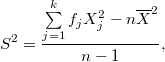
where  is the number of different values of
  and
and  is the frequency of the value
  of
of  . The standard deviation
  is the square root of the variance
  .
.
The variance and standard deviation show the deviation of the samples around the mean value. Small deviation from the mean demonstrates a strong central tendency of the samples. Large deviation reveals little central tendency and shows large statistical randomness.
Numerical estimates of the distribution parameters are required to reduce the family of distributions to a single distribution and test the corresponding hypothesis. Figure 14.1 describes estimators for the most common distributions occurring in network modelling. If  denotes a parameter, the estimator is denoted by
  . Except for an adjustment to remove bias in the estimates of
  for the normal distribution and in the estimate of
  of the uniform distribution, these estimators are the maximum likelihood estimators based on the sample data.
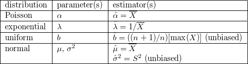
Probability distributions describe the random variations that occur in the real world. Although we call the variations random, randomness has different degrees; the different distributions correspond to how the variations occur. Therefore, different distributions are used for different simulation purposes. Probability distributions are represented by probability density functions. Probability density functions show how likely a certain value is. Cumulative density functions give the probability of selecting a number at or below a certain value. For example, if the cumulative density function value at 1 was equal to 0.85, then  of the time, selecting from this distribution would give a number less than 1. The value of a cumulative density function at a point is the area under the corresponding probability density curve to the left of that value. Since the total area under the probability density function curve is equal to one, cumulative density functions converge to one as we move toward the positive direction. In most of the modelling cases, the modeller does not need to know all details to build a simulation model successfully. He or she has only to know which distribution is the most appropriate one for the case.
Below, we summarise the most common statistical distributions. We use the simulation modelling tool COMNET to depict the respective probability density functions (PDF). From the practical point of view, a PDF can be approximated by a histogram with all the frequencies of occurrences converted into probabilities.
-
Normal distribution
It typically models the distribution of a compound process that can be described as the sum of a number of component processes. For instance, the time to transfer a file (response time) sent over the network is the sum of times required to send the individual blocks making up the file. In modelling tools the normal distribution function takes two positive, real numbers: mean and standard deviation. It returns a positive, real number. The stream parameter
 specifies which random number stream will be used to provide the sample. It is also often used to model message sizes. For example, a message could be described with mean size of 20,000 bytes and a standard deviation of 5,000 bytes.
 -
Poisson distribution
It models the number of independent events occurring in a certain time interval; for instance, the number of packets of a packet flow received in a second or a minute by a destination. In modelling tools, the Poisson distribution function takes one positive, real number, the mean. The “number” parameter in Figure 14.3 specifies which random number stream will be used to provide the sample. This distribution, when provided with a time interval, returns an integer which is often used to represent the number of arrivals likely to occur in that time interval. Note that in simulation, it is more useful to have this information expressed as the time interval between successive arrivals. For this purpose, the exponential distribution is used.
-
Exponential distribution
It models the time between independent events, such as the interarrival time between packets sent by the source of a packet flow. Note, that the number of events is Poisson, if the time between events is exponentially distributed. In modelling tools, the Exponential distribution function 14.4 takes one positive, real number, the mean and the stream parameter
 that specifies which random number stream will be used to provide the sample. Other application areas include: Time between data base transactions, time between keystrokes, file access, emails, name lookup request, HTTP lookup, X-window protocol exchange, etc.
 -
Uniform distribution
Uniform distribution models (see Figure 14.5) data that range over an interval of values, each of which is equally likely. The distribution is completely determined by the smallest possible value min and the largest possible value max. For discrete data, there is a related discrete uniform distribution as well. Packet lengths are often modelled by uniform distribution. In modelling tools the Uniform distribution function takes three positive, real numbers: min, max, and stream. The stream parameter x specifies which random number stream will be used to provide the sample.
-
Pareto distribution
The Pareto distribution (see 14.6) is a power-law type distribution for modelling bursty sources (not long-range dependent traffic). The distribution is heavily peaked but the tail falls off slowly. It takes three parameters: location, shape, and offset. The location specifies where the distribution starts, the shape specifies how quickly the tail falls off, and the offset shifts the distribution.
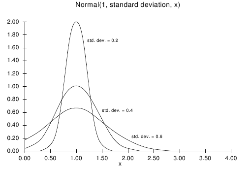
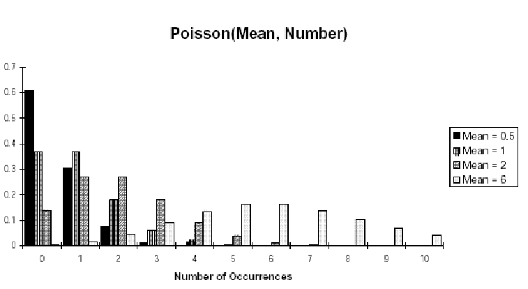
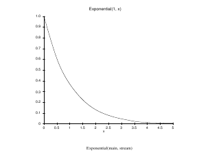
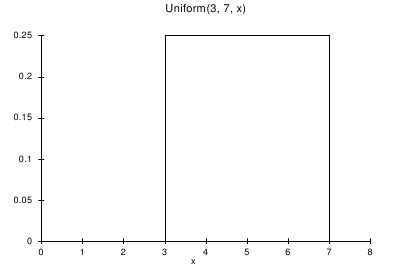
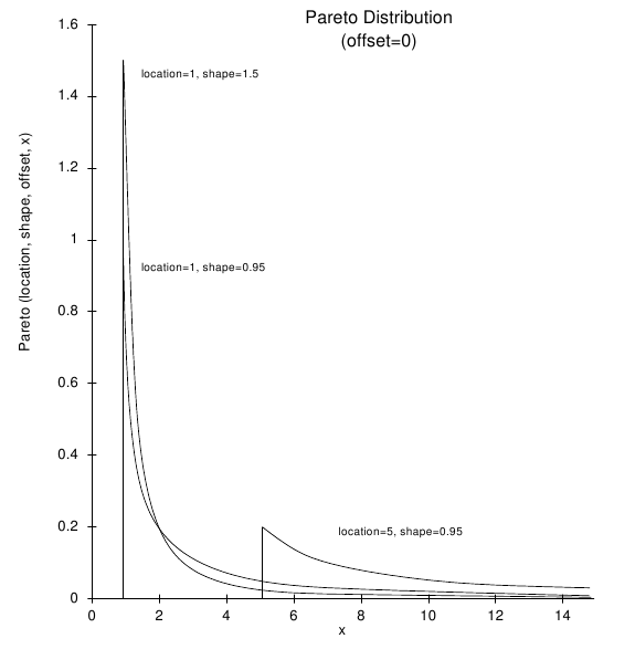
A common use of probability distribution functions is to define various network parameters. A typical network parameter for modelling purposes is the time between successive instances of messages when multiple messages are created. The specified time is from the start of one message to the start of the next message. As it is discussed above, the most frequent distribution to use for interarrival times is the exponential distribution (see Figure 14.7).
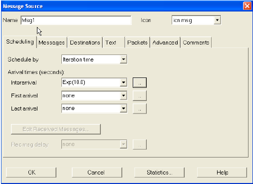
The parameters entered for the exponential distribution are the mean value and the random stream number to use. Network traffic is often described as a Poisson process. This generally means that the number of messages in successive time intervals has been observed and the distribution of the number of observations in an interval is Poisson distributed. In modelling tools, the number of messages per unit of time is not entered. Rather, the interarrival time between messages is required. It may be proven that if the number of messages per unit time interval is Poisson-distributed, then the interarrival time between successive messages is exponentially distributed. The interarrival distribution in the following dialog box for a message source in COMNET is defined by Exp (10.0). It means that the time from the start of one message to the start of the next message follows an exponential distribution with 10 seconds on the average. Figure 14.8 shows the corresponding probability density function.
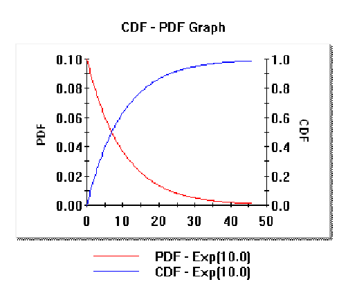
Many simulation models focus on the simulation of various traffic flows. Traffic flows can be simulated by either specifying the traffic characteristics as input to the model or by importing actual traffic traces that were captured during certain application transactions under study. The latter will be discussed in a subsequent section on Baselining.
Network modellers usually start the modelling process by first analysing the captured traffic traces to visualise network attributes. It helps the modeller understand the application level processes deep enough to map the corresponding network events to modelling constructs. Common tools can be used before building the model. After the preliminary analysis, the modeller may disregard processes, events that are not important for the study in question. For instance, the capture of traffic traces of a database transaction reveals a large variation in frame lengths. Figure 14.9 helps visualise the anomalies:
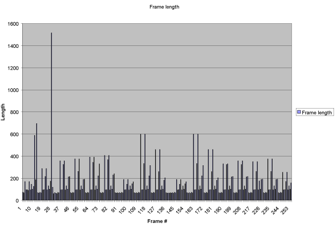
The analysis of the same trace (Figure 14.10) also discloses a large deviation of the interarrival times of the same frames (delta times):
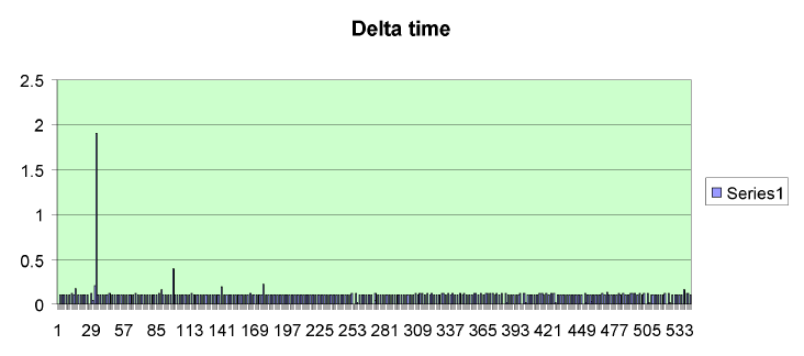
Approximating the cumulative probability distribution function by a histogram of the frame lengths of the captured traffic trace (Figure 14.11) helps the modeller determine the family of the distribution:
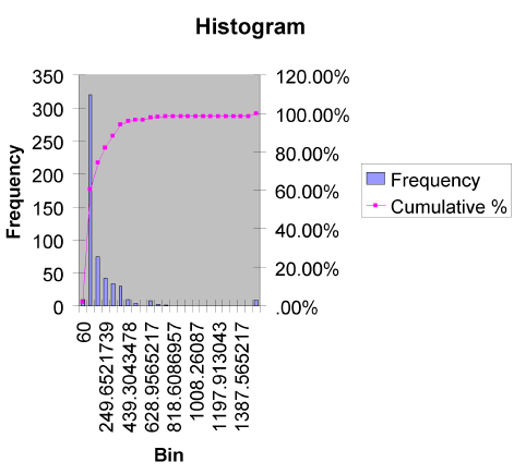
The section summaries the main features of the widely used discrete event simulation tools, OPNET and COMNET, and the supporting network analysers, Network Associates' Sniffer and OPNET's Application Characterisation Environment.
OPtimized Network Engineering Tools (OPNET) is a comprehensive simulation system capable of modelling communication networks and distributed systems with detailed protocol modelling and performance analysis. OPNET consists of a number of tools that fall into three categories corresponding to the three main phases of modelling and simulation projects: model specification, data collection and simulation, and analysis.
During model specification the network modeller develops a representation of the network system under study. OPNET implements the concept of model reuse, i.e., models are based on embedded models developed earlier and stored in model libraries. The model is specified at various levels of details using specification editors. These editors categorise the required modelling information corresponding to the hierarchical structure of an actual network system. The highest level editor, the Project Editor develops network models consisting of network topology, subnets, links, and node models specified in the Node Editor. The Node Editor describes nodes' internal architecture, functional elements and data flow between them. Node models in turn, consist of modules with process models specified by the Process Editor. The lowest level of the network hierarchy, the process models, describes the module's behaviour in terms of protocols, algorithms, and applications using finite state machines and a high-level language.
There are several other editors to define various data models referenced by process- or node-level models, e.g., packet formats and control information between processes. Additional editors create, edit, and view probability density functions (PDFs) to control certain events, such as the interarrival time of sending or receiving packets, etc. The model-specification editors provide a graphical interface for the user to manipulate objects representing the models and the corresponding processes. Each editor can specify objects and operations corresponding to the model's abstraction level. Therefore, the Project Editor specifies nodes and link objects of a network, the Node Editor specifies processors, queues, transmitters, and receivers in the network nodes, and the Process Editor specifies the states and transitions in the processes. Figure 14.12 depicts the abstraction level of each editor:
Figure 14.12. The three modelling abstraction levels specified by the Project, Node, and Process editors.
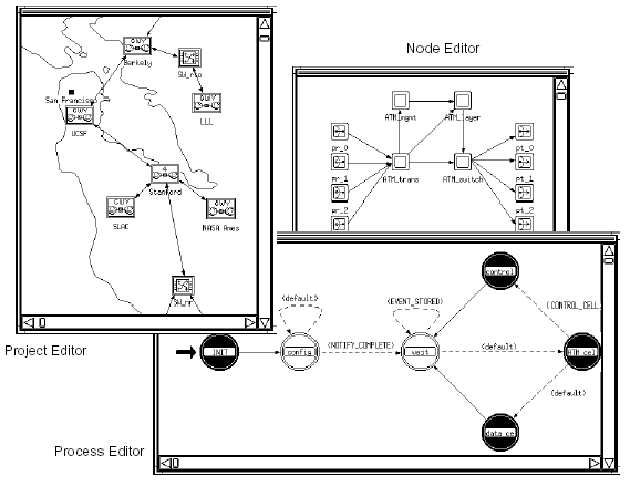
OPNET can produce many types of output during simulation depending on how the modeller defined the types of output. In most cases, modellers use the built in types of data: output vectors, output scalars, and animation:
-
Output vectors represent time-series simulation data consisting of list of entries, each of which is a time-value pair. The first value in the entries can be considered as the independent variable and the second as the dependent variable.
-
Scalar statistics are individual values derived from statistics collected during simulation, e.g., average transmission rate, peak number of dropped cells, mean response time, or other statistics.
-
OPNET can also generate animations that are viewed during simulation or replay after simulation. The modeller can define several forms of animations, for instance, packet flows, state transitions, and statistics.
Typically, much of the data collected during simulations is stored in output scalar and output vector files. In order to analyse these data OPNET provides the Analysis Tool which is a collection of graphing and numerical processing functions. The Analysis Tool presents data in the form of graphs or traces. Each trace consists of a list of abscissa  and ordinate
  pairs. Traces are held and displayed in analysis panels. The Analysis Tool supports a variety of methods for processing simulation output data and computing new traces. Calculations, such as histograms, PDF, CDF, and confidence intervals are included. Analysis Tool also supports the use of mathematical filters to process vector or trace data. Mathematical filters are defined as hierarchical block diagrams based on a predefined set of calculus, statistical, and arithmetic operators. The example diagrams below (Figures 14.13 and 14.14) shows graphs generated by the Analysis Tool:
Figure 14.13. Example for graphical representation of scalar data (upper graph) and vector data (lower graph).
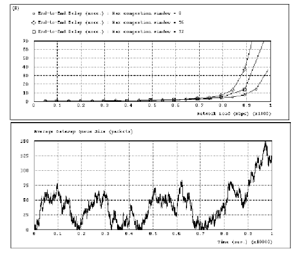
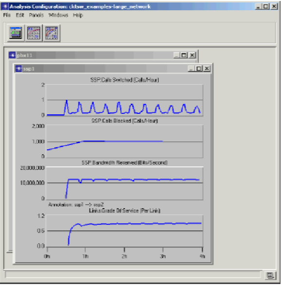
Figure 14.14 Analysis Tool Showing Four Graphs.
COMNET is another popular discrete-event simulation system. We will discuss it briefly and demonstrate its features in Section 14.9.
There is an increasing interest in predicting, measuring, modelling, and diagnosing application performance across the application lifecycle from development through deployment to production. Characterising the application's performance is extremely important in critical application areas, like in eCommerce. In the increasingly competitive eCommerce, the application's performance is critical, especially where the competition is just “one click” away. Application performance affects revenue. When an application performs poorly it is always the network that is blamed rather than the application. These performance problems may result from several areas including application design or slow database servers. Using tools, like ACE and Network Associates' Sniffer, network modellers can develop methodologies to identify the source of application slowdowns and resolve their causes. After analysing the applications, modellers can make recommendations for performance optimisation. The result is faster applications and better response times. The Application Characterisation Environment (ACE) is a tool for visualising, analysing, and troubleshooting network applications. Network managers and application developers can use ACE to
-
Locate network and application bottlenecks.
-
Diagnose network and application problems.
-
Analyse the affect of anticipated network changes on the response time of existing applications.
-
Predict application performance under varying configurations and network conditions
The performance of an application is determined by network attributes that are affected by the various components of a communication network. The following list contains some example for these attributes and the related network elements:
-
Network media
-
Bandwidth (Congestion, Burstiness)
-
Latency (TCP window size, High latency devices, Chatty applications)
-
-
Nodes
-
Clients
-
User time
-
Processing time
-
Starved for data
-
-
Servers
-
Processing time
-
Multi-tier waiting data
-
Starved for data
-
-
Application
-
Application turns (Too many turns – Chatty applications)
-
Threading (Single vs. multi-threaded)
-
Data profile (Bursty, Too much data processing)
-
Analysis of an application requires two phases:
-
Capture packet traces while an application is running to build a baseline for modelling an application. We can use the ACE's capturing tool or any other network analysers to capture packet traces. The packet traces can be captured by strategically deployed capture agents.
-
Import the capture file to create a representation of the application's transactions called an application task for further analysis of the messages and protocol data units generated by the application.
After creating the application task, we can perform the following operations over the captured traffic traces:
-
View and edit the captured packet traces on different levels of the network protocol stack in different windows. We can also use these windows to remove or delete sections of an application task. In this way, we focus on transactions of our interest.
-
Perform application level analysis by identifying and diagnosing bottlenecks. We can measure the components of the total response time in terms of application level time, processing time, and network time and view detailed statistics on the network and application. We can also decode and analyse the network and application protocol data units from the contents of the packet traces.
-
Predict application performance in “what-if” scenarios and for testing projected changes.
Without going into specific details we illustrate some of the features above through a simple three-tier application. We want to determine the reason or reasons of the slow response time from a Client that remotely accesses an Application Server (App Server) to retrieve information from a Database Server (DB Server). The connection is over an ADSL line between the client and the Internet, and a 100Mbps Ethernet connection between the App Server and the DB Server. We want to identify the cause of the slow response time and recommend solutions. We deployed capture agents at the network segments between the client and the App Server and between the servers. The agents captured traffic traces simultaneously during a transaction between the client and the App Server and the App Server and the DB Server respectively. Then, the traces were merged and synchronised to obtain the best possible analysis of delays at each tier and in the network.
After importing the trace into ACE, we can analyse the transaction in the Data Exchange Chart, which depicts the flow of application messages among tiers over time.
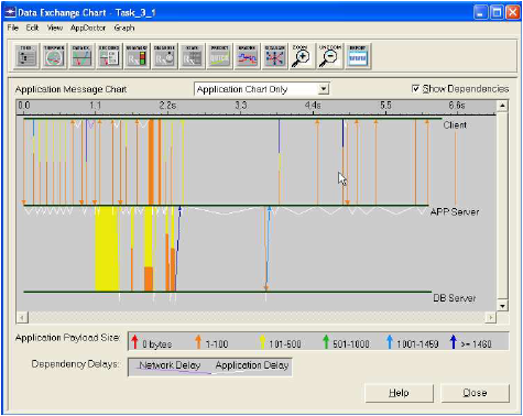
The Data Exchange Chart shows packets of various sizes being transmitted between the Client and the servers. The overall transaction response time is approximately 6 seconds. When the “Show Dependencies” checkbox is checked, the white dependency lines indicate large processing delays on the Application Server and Client tiers. For further analysis, we generate the “Summary of Delays” window showing how the total response time of the application is divided into four general categories: Application delay, Propagation delay, Transmission delay and Protocol/Congestion delay. Based on this chart we can see the relation between application and network related delays during the transaction between the client and the servers. The chart clearly shows that the application delay far outweighs the Propagation, Transmission, and Protocol/Congestion delays slowing down the transaction.
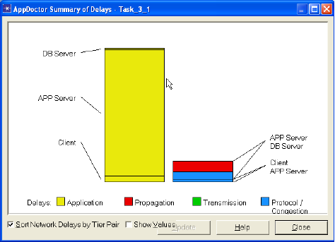
The “Diagnosis” function (Figure 14.17) provides a more granular analysis of possible bottlenecks by analysing factors that often cause performance problems in networked applications. Values over a specified threshold are marked as bottlenecks or potential bottlenecks.
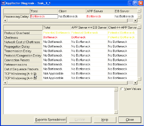
The diagnosis of the transaction confirms that the primary bottleneck is due to Processing Delay on the Application Server. The processing delay is due to the file I/O, CPU processing, or memory access. It also reveals another bottleneck: the chattiness of the application that leads us to the next step. We investigate the application behaviour in terms of application turns that can be obtained from the transaction statistics. An application turn is a change in direction of the application-message flow.
The statistics of the transaction (Figure 14.18) disclose that the number of application turns is high, i.e., the data sent by the transaction at a time is small. This may cause significant application and network delays. Additionally, a significant portion of application processing time can be spent processing the many requests and responses. The Diagnosis window indicates a “Chattiness” bottleneck without a “Network Cost of Chattiness” bottleneck, which means the following:
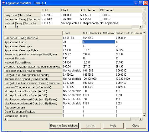
-
The application does not create significant network delays due to chattiness.
-
The application creates significant processing delays due to overhead associated with handling many small application level requests and responses.
-
The application's “Network Cost of Chattiness” could dramatically increase in a high-latency network.
The recommendation is that the application should send fewer, larger application messages. This will utilise network and tier resources more efficiently. For example, a database application should avoid sending a set of records one record at a time.
Would the response time decrease significantly if we added more bandwidth to the link between the client and the APP Server (Figure 14.19)? Answering this question is important because adding more bandwidth is expensive. Using the prediction feature we can answer the question. In the following chart we selected the bandwidth from 128K to 10Mbps. The chart shows that beyond approximately 827 Kbps there is no significant improvement in response time, i.e., for this application the recommended highest bandwidth is no more than 827Kbps, which can be provided by a higher speed DSL line.
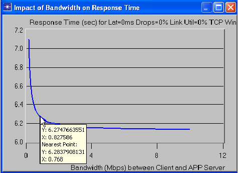
After the analysis of the application's performance, we can immediately create the starting baseline model from the captured traffic traces for further simulation studies as illustrated in Figure 14.20.
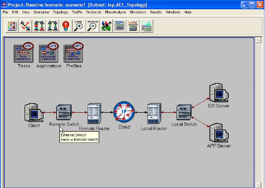
Another popular network analyser is Network Associates' Sniffer. (Network Associates has recently renamed it to Netasyst.) It is a powerful network visualisation tool consisting of a set of functions to:
-
Capture network traffic for detailed analysis.
-
Diagnose problems using the Expert Analyzer.
-
Monitor network activity in real time.
-
Collect detailed utilisation and error statistics for individual stations, conversations, or any portion of your network.
-
Save historical utilisation and error information for baseline analysis.
-
Generate visible and audible real-time alarms and notify network administrators when troubles are detected.
-
Probe the network with active tools to simulate traffic, measure response times, count hops, and troubleshoot problems.
For further details we refer the reader to the vendors' documentations on http://www.nai.com.
There are several approaches for network modelling. One possible approach is the creation of a starting model that follows the network topology and approximates the assumed network traffic statistically. After some changes are made, the modeller can investigate the impact of the changes of some system parameters on the network or application performance. This is an approach when it is more important to investigate the performance difference between two scenarios rather than starting from a model based on real network traffic. For instance, assuming certain client/server transactions, we want to measure the change of the response time as the function of the link utilisation 20%, 40%, 60%, etc. In this case it is not extremely important to start from a model based on actual network traffic. It is enough to specify certain amount of data transmission estimated by a frequent user or designer. We investigate, for this amount of data, how much the response time will increase as the link utilisation increases relative to the starting scenario.
The most common approach for network modelling follows the methodologies of proactive network management. It implies the creation of a network model using actual network traffic as input to simulate current and future behaviour of the network and predict the impact of the addition of new applications on the network performance. By making use of modelling and simulation tools network managers can change the network model by adding new devices, workstations, servers, and applications. Or they can upgrade the links to higher speed network connections and perform “what-if” scenarios before the implementation of the actual changes. We follow this approach in our further discussions because this approach has been widely accepted in the academia, corporate world, and the industry. In the subsequent paragraphs we elaborate a sequence of modelling steps, called the Model Development Life Cycle – MDLC that the author has applied in various real life scenarios of modelling large enterprise networks. The MDLC has the following steps:
-
Identification of the topology and network components.
-
Data collection.
-
Construction and validation of the baseline model. Perform network simulation studies using the baseline.
-
Creation of the application model using the details of the traffic generated by the applications.
-
Integration of the application and baseline model and completion of simulation studies.
-
Further data gathering as the network growths and changes and as we know more about the applications.
-
Repeat the same sequence.
In the following, we expand the steps above:
Identification of the topology and network components.
Topology data describes the physical network components (routers, circuits, and servers) and how they are connected. It includes the location and configuration description of each internetworking device, how those devices are connected (the circuit types and speeds), the type of LANs and WANs, the location of the servers, addressing schemes, a list of applications and protocols, etc.
Data collection.
In order to build the baseline model we need to acquire topology and traffic data. Modellers can acquire topology data either by entering the data manually or by using network management tools and network devices' configuration files. Several performance management tools use the Simple Network Management Protocol – SNMP to query the Management Information Base (MIB) maintained by SNMP agents running in the network's routers and other internetworking devices. This process is known as an SNMP discovery. We can import topology data from routers' configuration files to build a representation of the topology for the network in question. Some performance management tools can import data using the map file from a network management platform, such as HP OpenView or IBM NetView. Using the network management platform's export function, the map file can be imported by modelling.
The network traffic input to the baseline model can be derived from various sources: Traffic descriptions from interviews and network documents, design or maintenance documents, MIB/SNMP reports and network analyser and Remote Monitoring—traffic traces. RMON is a network management protocol that allows network information to be gathered at a single node. RMON traces are collected by RMON probes that collect data at different levels of the network architecture depending on the probe's standard. Figure 14.21 includes the most widely used standards and the level of data collection:
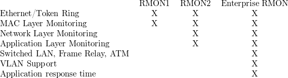
Network traffic can be categorised as usage-based data and application-based data. The primary difference between usage- and application-based data is the degree of details that the data provides and the conclusions that can be made based on the data. The division can be clearly specified by two adjacent OSI layers, the Transport layer and the Session layer: usage-based data is for investigating the performance issues through the transport layer; application-based data is for analysing the rest of the network architecture above the Transport layer. (In Internet terminology this is equivalent to the cut between the TCP level and the applications above the TCP level.)
The goal of collecting usage-based data is to determine the total traffic volume before the applications are implemented on the network. Usage-based data can be gathered from SNMP agents in routers or other internetworking devices. SNMP queries sent to the routers or switches provide statistics about the exact number of bytes that have passed through each LAN interface, WAN circuit, or (Permanent Virtual Circuit – PVC) interfaces. We can use the data to calculate the percentage of utilisation of the available bandwidth for each circuit.
The purpose of gathering application-based data is to determine the amount of data generated by an application and the type of demand the application makes. It allows the modeller to understand the behaviour of the application and to characterise the application level traffic. Data from traffic analysers or from RMON2-compatible probes, Sniffer, NETScout Manager, etc., provide specifics about the application traffic on the network. Strategically placed data collection devices can gather enough data to provide clear insight into the traffic behaviour and flow patterns of the network applications. Typical application level data collected by traffic analysers:
-
The type of applications.
-
Hosts communicating by network layer addresses (i.e., IP addresses).
-
The duration of the network conversation between any two hosts (start time and end time).
-
The number of bytes in both the forward and return directions for each network conversation.
-
The average size of the packets in the forward and return directions for each network conversation.
-
Traffic burstiness.
-
Packet size distributions.
-
Packet interarrival distributions.
-
Packet transport protocols.
-
Traffic profile, i.e., message and packet sizes, interarrival times, and processing delays.
-
Frequency of executing application for a typical user.
-
Major interactions of participating nodes and sequences of events.
Construction and validation of the baseline model. Perform network simulation studies using the baseline.
The goal of building a baseline model is to create an accurate model of the network as it exists today. The baseline model reflects the current “as is” state of the network. All studies will assess changes to the baseline model. This model can most easily be validated since its predictions should be consistent with current network measurements. The baseline model generally only predicts basic performance measures such as resource utilisation and response time.
The baseline model is a combination of the topology and usage-based traffic data that have been collected earlier. It has to be validated against the performance parameters of the current network, i.e., we have to prove that the model behaves similarly to the actual network activities. The baseline model can be used either for analysis of the current network or it can serve as the basis for further application and capacity planning. Using the import functions of a modelling tool, the baseline can be constructed by importing first the topology data gathered in the data collection phase of the modelling life cycle. Topology data is typically stored in topology files (.top or .csv) created by Network Management Systems, for instance HP OpenView or Network Associate's Sniffer. Traffic files can be categorised as follows:
-
Conversation pair traffic files that contain aggregated end-to-end network load information, host names, packet counts, and byte counts for each conversation pair. The data sets allow the modelling tool to preserve the bursty nature of the traffic. These files can be captured by various data collection tools.
-
Event trace traffic files that contain network load information in the form of individual conversations on the network rather than summarised information. During simulation the file can replay the captured network activity on an event by event basis.
Before simulation the modeller has to decide on the following simulation parameters:
-
Run length: Runtime length must exceed the longest message delay in the network. During this time the simulation should produce sufficient number of events to allow the model to generate enough samples of every event.
-
Warm-up period: The simulation warm-up period is the time needed to initialise packets, buffers, message queues, circuits, and the various elements of the model. The warm-up period is equal to a typical message delay between hosts. Simulation warm-up is required to ensure that the simulation has reached steady-state before data collection begins.
-
Multiple replications: There may be a need for multiple runs of the same model in cases when statistics are not sufficiently close to true values. We also need multiple runs prior to validation when we execute multiple replicates to determine variation of statistics between replications. A common cause of variation between replications is rare events.
-
Confidence interval: A confidence interval is an interval used to estimate the likely size of a population parameter. It gives an estimated range of values that has a specified probability of containing the parameter being estimated. Most commonly used intervals are the 95% and 99% confidence intervals that have .95 and .99 probabilities respectively of containing the parameter. In simulation, confidence interval provides an indicator of the precision of the simulation results. Fewer replications result in a broader confidence interval and less precision.
In many modelling tools, after importing both the topology and traffic files, the baseline model is created automatically. It has to be checked for construction errors prior to any attempts at validation by performing the following steps:
-
Execute a preliminary run to confirm that all source-destination pairs are present in the model.
-
Execute a longer simulation with warm-up and measure the sent and received message counts and link utilisation to confirm that correct traffic volume is being transmitted.
Validating the baseline model is the proof that the simulation produces the same performance parameters that are confirmed by actual measurements on the physical network. The network parameters below can usually be measured in both the model and in the physical network:
-
Number of packets sent and received
-
Buffer usage
-
Packet delays
-
Link utilisation
-
Node's CPU utilisation
Confidence intervals and the number of independent samples affect how close a match between the model and the real network is to be expected. In most cases, the best that we can expect is an overlap of the confidence interval of predicted values from the simulation and the confidence interval of the measured data. A very close match may require too many samples of the network and too many replications of the simulation to make it practical.
Creation of the application model using the details of the traffic generated by the applications.
Application models are studied whenever there is a need to evaluate the impact of a networked application on the network performance or to evaluate the application's performance affected by the network. Application models provide traffic details between network nodes generated during the execution of the application. The steps of building an application model are similar to the ones for baseline models.
-
Gather data on application events and user profiles.
-
Import application data into a simulation model manually or automatically.
-
Identify and correct any modelling errors.
-
Validate the model.
Integration of the application and baseline models and completion of simulation studies.
The integration of the application model(s) and baseline model follows the following steps:
-
Start with the baseline model created from usage-based data.
-
Use the information from the application usage scenarios (locations of users, number of users, transaction frequencies) to determine where and how to load the application profiles onto the baseline model.
-
Add the application profiles generated in the previous step to the baseline model to represent the additional traffic created by the applications under study.
Completion of Simulation studies consists of the following steps:
-
Use a modelling tool to run the model or simulation to completion.
-
Analyse the results: Look at the performance parameters of the target transactions in comparison to the goals established at the beginning of the simulation.
-
Analyse the utilisation and performance of various network elements, especially where the goals are not being met.
Typical simulation studies include the following cases:
-
Capacity analysis
Capacity analysis studies the changes of network parameters, for instance:
-
Changes in the number and location of users.
-
Changes in network elements capacity.
-
Changes in network technologies.
A modeller may be interested in the effect of the changes above on the following network parameters:
-
Switches and routers' utilisation
-
Communications link utilisation
-
Buffer utilisation
-
Retransmitted and lost packets
-
-
Response time analysis
The scope of response time analysis is the study of message and packet transmission delay:
-
Application and network level packet end-to-end delay.
-
Packet round trip delay.
-
Message/packet delays.
-
Application response time.
-
-
Application Analysis
The scope of application studies is the ratio of the total application response time relative to the individual components of network and application delay. Application's analysis provides statistics of various measures of network and application performance in addition to the items discussed in a previous section.
Further data gathering as the network growths and as we know more about the applications
The goal of this phase is to analyse or predict how a network will perform both under current conditions and when changes to traffic load (new applications, users, or network structure) are introduced:
-
Identify modifications to the network infrastructure that will alter capacity usage of the network's resources.
-
A redesign can include increasing or decreasing capacity, relocating network elements among existing network sites, or changing communications technology.
-
Modify the models to reflect these changes.
-
Assess known application development or deployment plans in terms of projected network impact.
-
Assess business conditions and plans in terms of their impact on the network from projected additional users, new sites, and other effects of the plans.
-
Use ongoing Baselining techniques to watch usage trends over time, especially related to Internet and intranet usage.
Recent measurements of local area network traffic and wide-area network traffic have proved that the widely used Markovian process models cannot be applied for today's network traffic. If the traffic were a Markovian process, the traffic's burst length would be smoothed by averaging over a long time scale, contradicting the observations of today's traffic characteristics. Measurements of real traffic also prove that traffic burstiness is present on a wide range of time scales. Traffic that is bursty on many or all time scales can be characterised statistically using the concept of self-similarity. Selfsimilarity is often associated with objects in fractal geometry, objects that appear to look alike regardless of the scale at which they are viewed. In case of stochastic processes like time series, the term self-similarity refers to the process' distribution, which, when viewed at varying time scales, remains the same. Self-similar time series has noticeable bursts, which have long periods with extremely high values on all time scales. Characteristics of network traffic, such as packets/sec, bytes/sec, or length of frames, can be considered as stochastic time series. Therefore, measuring traffic burstiness is the same as characterising the self-similarity of the corresponding time series.
The self-similarity of network traffic has also been observed in studies in numerous papers. These and other papers show that packet loss, buffer utilisation, and response time are totally different when simulations use either real traffic data or synthetic data that include self-similarity.
Background.
Let  be a covariance stationary stochastic process. Such a process has a constant mean
  , finite variance
  , and an autocorrelation function
  , that depends only on
  . It is assumed that
  has an autocorrelation function of the form:

where  and
and  is a positive constant. Let
  represent a new time series obtained by averaging the original series
  over nonoverlapping blocks of size
  . For each
  is specified by
  . Let
. Let  denote the autocorrelation function of the aggregated time series
  .
.
Definition of self-similarity.
The process  called exactly self-similar with self-similarity parameter
  if the corresponding aggregated processes
  have the same correlation structure as
  , i.e.
  for all
  .
.
A covariance stationary process  is called asymptotically self-similar with self-similarity parameter
  , if for all
  large enough
  , as
, as  ,
,  .
.
Definition of long-range dependency.
A stationary process is called long-range dependent if the sum of the autocorrelation values approaches infinity:  . Otherwise, it is called short-range dependent. It can be derived from the definitions that while short-range dependent processes have exponentially decaying autocorrelations, the autocorrelations of long-range dependent processes decay hyperbolically; i.e., the related distribution is heavy-tailed. In practical terms, a random variable with heavy-tail distribution generates extremely large values with high probability. The degree of self-similarity is expressed by the parameter
  or Hurst-parameter. The parameter represents the speed of decay of a process' autocorrelation function. As
  the extent of both self-similarity and long-range dependence increases. It can also be shown that for self-similar processes with long-range dependency
  .
.
Traffic models.
Traffic modelling originates in traditional voice networks. Most of the models have relied on the assumption that the underlying processes are Markovian (or more general, short-range dependent). However, today's high-speed digital packet networks are more complex and bursty than traditional voice traffic due to the diversity of network services and technologies.
Several sophisticated stochastic models have been developed as a reaction to new developments, such as Markov-modulated Poisson processes, fluid flow models, Markovian arrival processes, batched Markovian arrival process models, packet train models, and Transform-Expand-Sample models. These models mainly focus on the related queueing problem analytically. They are usually not compared to real traffic patterns and not proven to match the statistical property of actual traffic data.
Another category of models attempts to characterise the statistical properties of actual traffic data. For a long time, the area of networking research has lacked adequate traffic measurements. However, during the past years, large quantities of network traffic measurements have become available and collected in the Web and high-speed networks. Some of these data sets consist of high-resolution traffic measurements over hours, days, or weeks. Other data sets provide information over time periods ranging from weeks to months and years. Statistical analyses of these high time-resolution traffic measurements have proved that actual traffic data from packet networks reveal self-similarity. These results point out the difference between traditional models and measured traffic data. While the assumed processes in traditional packet traffic models are short-range dependent, measured packet traffic data show evidence of long-range dependency. Figure 14.22 illustrates the difference between Internet traffic and voice traffic for different numbers of aggregated users. As the number of voice flows increases, the traffic becomes more and more smoothed contrary to the Internet traffic.
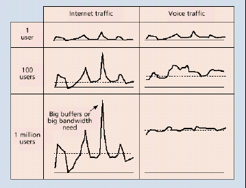
Quite the opposite to the well developed field of short-range dependent queueing models, fewer theoretical results exist for queueing systems with long-range dependence. For some of the results. In terms of modelling, the two major groups of self-similar models are fractional Gaussian noises and fractional ARIMA processes. The Gaussian models accurately represent aggregation of many traffic streams. Another well-known model, the M/Pareto model has been used in modelling network traffic that is not sufficiently aggregated for the Gaussian model to apply.
Black box vs. structural models.
We share the opinion calling the approach of traditional time series analysis as black box modelling as opposite to the structural modelling that concentrates on the environment in which the models' data was collected; i.e., the complex hierarchies of network components that make up today's communications systems. While the authors admit that black box models can be and are useful in other contexts, they argue that black box models are of no use for understanding the dynamic and complex nature of the traffic in modern packet networks. Black box models have not much use in designing, managing and controlling today's networks either. In order to provide physical explanations for empirically observed phenomena such as long-range dependency, we need to replace black box models with structural models. The attractive feature of structural traffic models is that they take into account the details of the layered architecture of today's networks and can analyse the interrelated network parameters that ultimately determine the performance and operation of a network. Time series models usually handle these details as black boxes. Because actual networks are complex systems, in many cases, black box models assume numerous parameters to represent a real system accurately. For network designers, who are important users of traffic modelling, black box models are not very useful. It is rarely possible to measure or estimate the model's numerous parameters in a complex network environment. For a network designer, a model ought to be simple, meaningful in a particular network. It can relay on actual network measurements, and the result ought to be relevant to the performance and the operation of a real network.
For a long time, traffic models were developed independently of traffic data collected in real networks. These models could not be applied in practical network design. Today the availability of huge data sets of measured network traffic and the increasing complexity of the underlying network structure emphasise the application of the Ockham' Razer in network modelling. (Ockham's Razor is a principle of the mediaeval philosopher William Ockham. According to his principle, modellers should not make more assumptions than the minimum needed. This principle is also called the Principle of Parsimony and motivates all scientific modelling and theory building. It states that modellers should choose the simplest model among a set of otherwise equivalent models of a given phenomenon. In any given model, Ockham's Razor helps modellers include only those variables that are really needed to explain the phenomenon. Following the principle, model development will become easier, reducing the possibilities for inconsistencies, ambiguities and redundancies.)
Structural models are presented, for instance in different papers, which demonstrate how the self-similar nature of aggregated network traffic of all conversations between hosts explains the details of the traffic dynamics at the level generated by the individual hosts. The papers introduce structural traffic models that have a physical meaning in the network context and underline the predominance of long-range dependence in the packet arrival patterns generated by the individual conversations between hosts. The models provide insight into how individual network connections behave in local and wide area networks. Although the models go beyond the black box modelling methodology by taking into account the physical structure of the aggregated traffic patterns, they do not include the physical structure of the intertwined structure of links, routers, switches, and their finite capacities along the traffic paths.
Crovella and Stavros demonstrated that World Wide Web traffic shows characteristics that are consistent with self-similarity. They show that transmission times may be heavy tailed, due to the distribution of available file sizes in the Web. It is also shown that silent times may also be heavy-tailed; primarily due to the effect of user “think time”. Similarly to the structural models due to Willinger at al., their paper lacks of analysing the impact of selfsimilar traffic on the parameters of the links and the routers' buffers that ultimately determine a network's performance.
This chapter describes a traffic model that belongs to the structural model category above. We implement the M/Pareto model within the discrete event simulation package COMNET that allows the analysis of the negative impact of self-similar traffic on not just one single queue, but on the overall performance of various interrelated network components, such as link, buffers, response time, etc. The commercially available package does not readily provide tools for modelling self-similar, long-range dependent network traffic. The model-generated traffic is based on measurements collected from a real ATM network. The choice of the package emphasises the need for integrated tools that could be useful not just for theoreticians, but also for network engineers and designers. Our paper intends to narrow the gap between existing, well-known theoretical results and their applicability in everyday, practical network analysis and modelling. It is highly desirable that appropriate traffic models should be accessible from measuring, monitoring, and controlling tools. Our model can help network designers and engineers, the ultimate users of traffic modelling, understand the dynamic nature of network traffic and assist them to design, measure, monitor, and control today's complex, high-speed networks in their everyday's practice.
Implications of burstiness on high-speed networks.
Various papers discuss the impact of burstiness on network congestion. Their conclusions are:
-
Congested periods can be quite long with losses that are heavily concentrated.
-
Linear increases in buffer size do not result in large decreases in packet drop rates.
-
A slight increase in the number of active connections can result in a large increase in the packet loss rate.
Results show that packet traffic “spikes” (which cause actual losses) ride on longerterm “ripples”, which in turn ride on still longer-term “swells”.
Another area where burstiness can affect network performance is a link with priority scheduling between classes of traffic. In an environment, where the higher priority class has no enforced bandwidth limitations (other than the physical bandwidth), interactive traffic might be given priority over bulk-data traffic. If the higher priority class is bursty over long time scales, then the bursts from the higher priority traffic could obstruct the lower priority traffic for long periods of time.
The burstiness may also have an impact on networks where the admission control mechanism is based on measurements of recent traffic, rather than on policed traffic parameters of individual connections. Admission control that considers only recent traffic patterns can be misled following a long period of fairly low traffic rates.
Each transaction between a client and a server consists of active periods followed by inactive periods. Transactions consist of groups of packets sent in each direction. Each group of packets is called a burst. The burstiness of the traffic can be characterised by the following time parameters:
-
Transaction Interarrival Time (TIAT): The time between the first packet in a transaction and the first packet of the next immediate transaction.
-
Burst Interarrival Time,
 ,
,  arrival rate of bursts: The time between bursts.
 -
Packet Interarrival Time,
 ,
,  : arrival rate of packets: The time between packets in a burst.
It is anticipated that the rapid and ongoing aggregation of more and more traffic onto integrated multiservice networks will eventually result in traffic smoothing. Once the degree of aggregation is sufficient, the process can be modelled by Gaussian process. Currently, network traffic does not show characteristics that close to Gaussian. In many networks the degree of aggregation is not enough to balance the negative impact of bursty traffic. However, before traffic becomes Gaussian, existing methods can still provide accurate measurement and prediction of bursty traffic.
Most of the methods are based on the estimate of the Hurst parameter  - the higher the value of H, the higher the burstiness, and consequently, the worse the queueing performance of switches and routers along the traffic path. Some are more reliable than others. The reliability depends on several factors; e.g., the estimation technique, sample size, time scale, traffic shaping or policing, etc. Based on published measurements we investigated methods with the smallest estimation error*.
Footnote. Variance, Aggregated Variance, Higuchi, Variance of Residuals, Rescaled Adjusted Range (R/S), Whittle Estimator, Periodogram, Residuals of Regression.
Among those, we chose the Rescaled Adjusted Range (R/S) method because we found it implemented in the Benoit package. The Hurst parameter calculated by the package is input to our method.
Recent results have proven that the M/Pareto model is appropriate for modelling long-range dependent traffic flow characterised by long bursts. Originally, the model was introduced and applied in the analysis of ATM buffer levels. The M/Pareto model was also used to predict the queueing performance of Ethernet, VBR video, and IP packet streams in a single server queue. We apply the M/Pareto model not just for a single queue, but also for predicting the performance of an interconnected system of links, switches and routers affecting the individual network elements' performance.
The M/Pareto model is a Poisson process of overlapping bursts with arrival rate  . A burst generates packets with arrival rate
  . Each burst, from the time of its interval, will continue for a Pareto-distributed time period. The use of Pareto distribution results in generating extremely long bursts that characterise long-range dependent traffic.
The probability that a Pareto-distributed random variable  exceeds threshold
  is:
is:

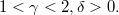
The mean of  , the mean duration of a burst
 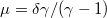 and its variance is infinite. Assuming a
  time interval, the mean number of packets
  in the time interval
  is:
is:

where

The M/Pareto model is asymptotically self-similar and it is shown that for the Hurst parameter the following equation holds:

We implemented the Hurst parameter and a modified version of the M/Pareto model in the discrete event simulation system COMNET. By using discrete event simulation methodology, we can get realistic results in measuring network parameters, such as utilisation of links and the queueing performance of switches and routers. Our method can model and measure the harmful consequences of aggregated bursty traffic and predict its impact on the overall network's performance.
In order to build the baseline model, we collected traffic traces in a large corporate network by the Concord Network Health network analyser system. We took measurements from various broadband and narrow band links including 45Mbps ATM, 56Kbps, and 128 Kbps frame relay connections. The Concord Network Health system can measure the traffic in certain time intervals at network nodes, such as routers and switches. We set the time intervals to 6000 seconds and measured the number of bytes and packets sent and received per second, packet latency, dropped packets, discard eligible packets, etc. Concord Network Health cannot measure the number of packets in a burst and the duration of the bursts as it is assumed in the M/Pareto model above. Due to this limitation of our measuring tool, we slightly modify our traffic model according to the data available. We took snapshots of the traffic in every five minutes from a narrow band frame relay connection between a remote client workstation and a server at the corporate headquarters as traffic destination in the following format:
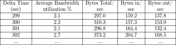
The mean number of bytes, the message delay from the client to server, the input buffer level at the client's local router, the number of blocked packets, the mean utilisations of the 56Kbps frame relay, the DS-3 segment of the ATM network, and the 100Mbps Ethernet link at the destination are summarised in Figure 14.24.
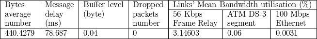
COMNET represents a transaction by a message source, a destination, the size of the message, communication devices, and links along the path. The rate at which messages are sent is specified by an interarrival time distribution, the time between two consecutive packets. The Poisson distribution in the M/Pareto model generates bursts or messages with arrival rate  , the number of arrivals, which are likely to occur in a certain time interval. In simulation, this information is expressed by the time interval between successive arrivals
  . For this purpose, we use the Exponential distribution. Using the Exponential distribution for interarrival time will result in an arrival pattern characterised by the Poisson distribution. In COMNET, we implemented the interarrival time with the function Exp(
 ). The interarrival time in the model is set to one second matching the sampling time interval set in Concord Network Health and corresponding to an arrival rate
  /sec.
/sec.
In the M/Pareto model, each burst continues for a Pareto-distributed time period. The Concord Network Health cannot measure the duration of a burst; hence, we assume that a burst is characterised by the number of bytes in a message sent or received in a second. Since the ATM cell rate algorithm ensures that equal length messages are processed in equal time, then longer messages require longer processing time. So we can say that the distribution of the duration of bursts is the same as the distribution of the length of bursts. Hence, we can modify the M/Pareto model by substituting the Pareto-distributed duration of bursts with the Pareto-distributed length of bursts. We derive  of the Pareto distribution not from the mean duration of bursts, but from the mean length of bursts.
The Pareto distributed length of bursts is defined in COMNET by two parameters- the location and the shape. The location parameter corresponds to the  , the shape parameter corresponds to the
  parameter of the M/Pareto model in (1) and can be calculated from the relation (4) as

The Pareto distribution can have infinite mean and variance. If the shape parameter is greater than 2, both the mean and variance are finite. If the shape parameter is greater than 1, but less than or equal to 2, the mean is finite, but then the variance is infinite. If the shape parameter is less than or equal to 1, both the mean and variance are infinite.
From the mean of the Pareto distribution we get:

The relations (5) and (6) allow us to model bursty traffic based on real traffic traces by performing the following steps:
-
a. Collect traffic traces using the Concord Network Health network analyser.
-
b. Compute the Hurst parameter
 by making use of the Benoit package with the traffic trace as input.
 -
c. Use the Exponential and Pareto distributions in the COMNET modelling tool with the parameters calculated above to specify the distribution of the interarrival time and length of messages.
-
d. Generate traffic according to the modified M/Pareto model and measure network performance parameters.
The traffic generated according to the steps above is bursty with parameter H calculated from real network traffic.
We validate our baseline model by comparing various model parameters of a 56Kbps frame relay and a 6Mbps ATM connection with the same parameters of a real network as the Concord Network Health network analyser traced it. For simplicity, we use only the “Bytes Total/sec” column of the trace, i.e., the total number of bytes in the “Bytes Total/sec” column is sent in one direction only from the client to the server. The Hurst parameter of the real traffic trace is  calculated by the Benoit package. The topology is as follows:
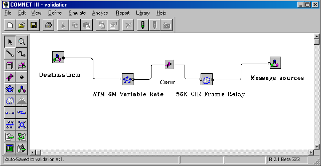
The “Message sources” icon is a subnetwork that represents a site with a token ring network, a local router, and a client  sending messages to the server
  in the “Destination” subnetwork:
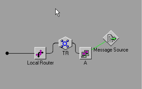
The interarrival time and the length of messages are defined by the Exponential and Pareto functions Exp (1) and Par (208.42, 1.9) respectively. The Pareto distribution's location (208.42) and shape (1.9) are calculated from formulas (5) and (6) by substituting the mean length of bursts (440 bytes from Table 2.) and  .
.
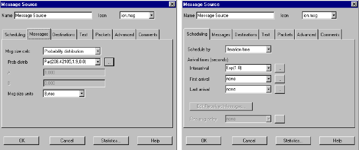
The corresponding heavy-tailed Pareto probability distribution and cumulative distribution functions are illustrated in Figure 14.28 (The  represents the number of bytes):
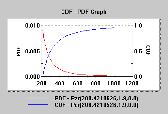
The “Frame Relay” icon represents a frame relay cloud with 56K committed information rate (CIR). The “Conc” router connects the frame relay network to a 6Mbps ATM network with variable rate control (VBR) as shown in Figures 14.29 and 14.30:
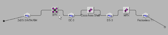
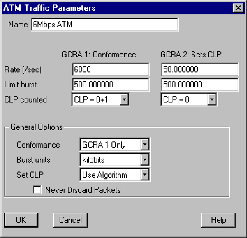
The “Destination” icon denotes a subnetwork with server  :
:
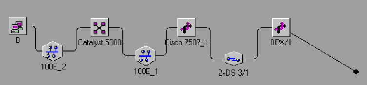
The results of the model show almost identical average for the utilisation of the frame relay link ( ) and the utilisation of the real measurements (3.1%):
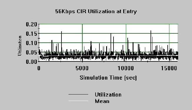
The message delay in the model is also very close to the measured delay between the client and the server (78 msec):
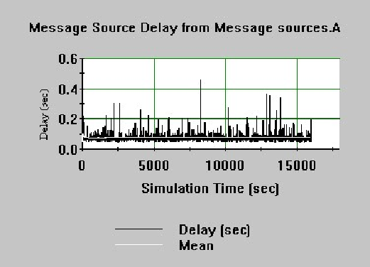
The input buffer level of the remote client's router in the model is almost identical with the measured buffer level of the corresponding router:
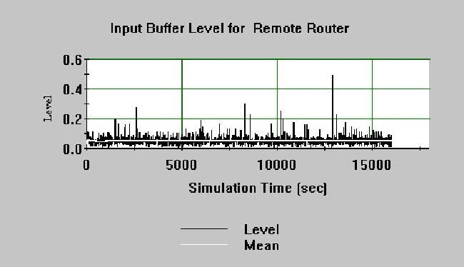
Similarly, the utilisations of the model's DS-3 link segment of the ATM network and the Ethernet link in the destination network closely match with the measurements of the real network:
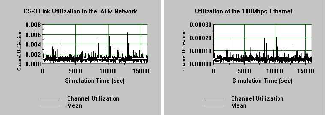
It can also be shown from the model's traffic trace that for the model generated messages the Hurst parameter  , i.e., the model generates almost the same bursty traffic as the real network. Furthermore, the number of dropped packets in the model was zero similarly to the number of dropped packets in the real measurements. Therefore, we start from a model that closely represents the real network.
In order to illustrate our method, we developed a COMNET simulation model to measure the consequences of bursty traffic on network links, message delays, routers' input buffers, and the number of dropped packets due to the aggregated traffic of large number of users. The model implements the Hurst parameter as it has been described in Section 3. We repeated the simulation for 6000 sec, 16000 sec and 18000 sec to allow infrequent events to occur a reasonable number of times. We found that the results are very similar in each simulation.
The “Message Source” subnetworks transmit messages as in the baseline model above, but with different burstiness:  , and with fixed size. Initially, we simulate four subnetworks and four users per subnetwork each sending the same volume of data (mean 440 bytes per second) as in the validating model above:
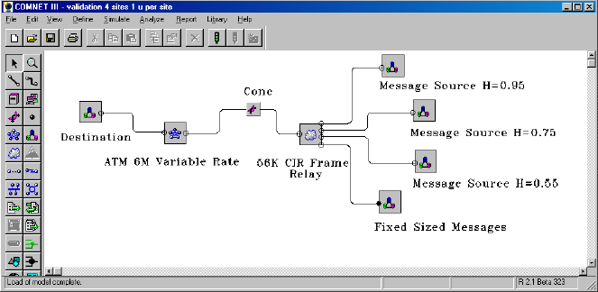
First, we are going to measure and illustrate the extremely high peaks in frame relay link utilisation and message delay. The model traffic is generated with message sizes determined by various Hurst parameters and fixed size messages for comparison. The COMNET modelling tool has a trace option to capture its own model generated traffic. It has been verified that for the model-generated traffic flows with various Hurst parameters the Benoit package computed similar Hurst parameters for the captured traces.
The following table shows the simulated average and peak link utilisation of the different cases. The utilisation is expressed in the [0, 1] scale not in percentages:
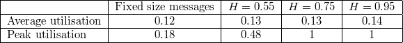
The enclosed charts in Appendix A clearly demonstrate that even though the average link utilisation is almost identical, the frequency and the size of the peaks increase with the burstiness, causing cell drops in routers and switches. We received the following results for response time measurements:
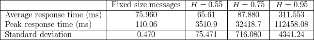
The charts in the Appendix A graphically illustrate the relation between response times and various Hurst parameters.
We also measured the number of cells dropped at a router's input buffer in the ATM network due to surge of bursty cells. We simulated the aggregated traffic of approximately 600 users each sending the same number of bytes in a second as in the measured real network. The number of blocked packets is summarised in the following table:
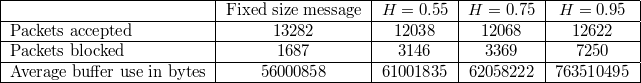
Theis chapter presented a discrete event simulation methodology to measure various network performance parameters while transmitting bursty traffic. It has been proved in recent studies that combining bursty data streams will also produce bursty combined data flow. The studies imply that the methods and models used in traditional network design require modifications. We categorise our modelling methodology as a structural model contrary to a black box model. Structural models focus on the environment in which the models' data was collected; i.e., the complex hierarchies of network components that make up today's communications systems. Although black box models are useful in other contexts, they are not easy to use in designing, managing and controlling today's networks. We implemented a well-known model, the M/Pareto model within the discrete event simulation package COMNET that allows the analysis of the negative impact of self-similar traffic on not just one single queue, but on the overall performance of various interrelated network components as well. Using real network traces, we built and validated a model by which we could measure and graphically illustrate the impact of bursty traffic on link utilisation, message delays, and buffer performance of Frame Relay and ATM networks. We illustrated that increasing burstiness results in extremely high link utilisation, response time, and dropped packets, and measured the various performance parameters by simulation.
The choice of the package emphasises the need for integrated tools that could be useful not just for theoreticians, but also for network engineers and designers. Our paper intends to narrow the gap between existing, well-known theoretical results and their applicability in everyday, practical network analysis and modelling. It is highly desirable that appropriate traffic models should be accessible from measuring, monitoring, and controlling tools. Our model can help network designers and engineers, the ultimate users of traffic modelling, understand the dynamic nature of network traffic and assist them in their everyday practice.
The following charts demonstrate that even though the average link utilisation for the various Hurst parameters is almost identical, the frequency and the size of the peaks increase with the burstiness, causing cell drops in routers and switches. The utilisation is expressed in the [0, 1] scale not in percentages:
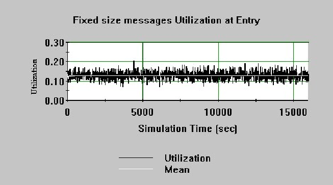
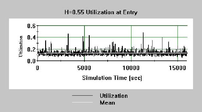
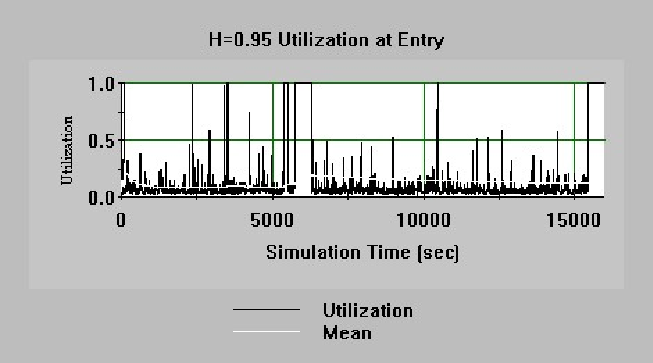
Figures 14.43–14.45 illustrate the relation between response time and various Hurst parameters:
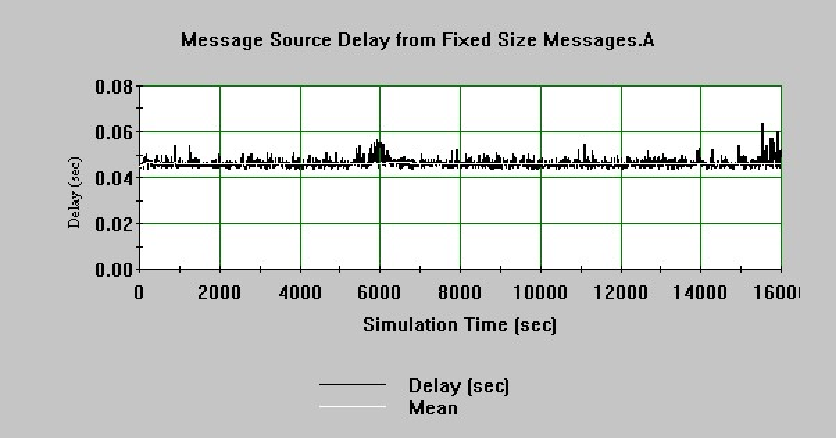
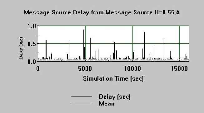
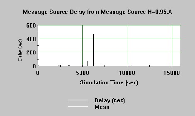
Exercises
14.9-1 Name some attributes, events, activities and state variables that belong to the following concepts:
-
Server
-
Client
-
Ethernet
-
Packet switched network
-
Call set up in cellular mobile network
-
TCP Slow start algorithm
14.9-2 Read the article about the application of the network simulation and write a report about how the article approaches the validation of the model.
14.9-3 For this exercise it is presupposed that there is a network analyser software (e.g., LAN Analyzer for Windows or any similar) available to analyse the network traffic. We use the mentioned software thereinafter.
-
Let's begin to transfer a file between a client and a server on the LAN. Observe the detailed statistics of the utilisation of the datalink and the number of packets per second then save the diagram.
-
Read the Capturing and analysing Packet chapter in the Help of LAN Analyzer.
-
Examine the packets between the client and the server during the file transfer.
-
Save the captured trace information about the packets in .csv format. Analyse this file using spreadsheet manager. Note if there are any too long time intervals between two packets, too many bad packets, etc. in the unusual protocol events.
14.9-4 In this exercise we examine the network analysing and baseline maker functions of the Sniffer. The baseline defines the activities that characterise the network. By being familiar with this we can recognise the non-normal operation. This can be caused by a problem or the growing of the network. Baseline data has to be collected in case of typical network operation. For statistics like bandwidth utilization and number of packets per second we need to make a chart that illustrates the information in a given time interval. This chart is needed because sampled data of a too short time interval can be false. After adding one or more network component a new baseline should be made, so that later the activities before and after the expansion can be compared. The collected data can be exported to be used in spreadsheet managers and modelling tools, that provides further analysing possibilities and is helpful in handling gathered data.
Sniffer is a very effective network analysing tool. It has several integrated functions.
-
Gathering traffic-trace information for detailed analysis.
-
Problem diagnosis with Expert Analyzer.
-
Real-time monitoring of the network activities.
-
Collecting detailed error and utilization statistics of nodes, dialogues or any parts of the network.
-
Storing the previous utilization and fault information for baseline analysis.
-
When a problem occurs it creates visible or audible alert notifications for the administrators.
-
For traffic simulation monitoring of the network with active devices, measuring the response time, hop counting and faults detection.
-
The Histroy Samples option of the Monitor menu allows us to record the network activities within a given time interval. This data can be applied for baseline creation that helps to set some thresholds. In case of non-normal operation by exceeding these thresholds some alerts are triggered. Furthermore this data is useful to determine the long-period alteration of the network load, therefore network expansions can be planned forward.
-
Maximum 10 of network activities can be monitored simultaneously. Multiple statistics can be started for a given activity, accordingly short-period and long-period tendencies can be analysed concurrently. Network activities that are available for previous statistics depends on the adapter selected in the Adapter dialogue box. For example in case of a token ring network the samples of different token ring frame types (e.g, Beacon frames), in Frame Relay networks the samples of different Frame Relay frame types (e.g, LMI frames) can be observed. The available events depend on the adapter.
Practices:
-
Set up a filter (Capture/Define filter) between your PC and a remote Workstation to sample the IP traffic.
-
Set up the following at the Monitor/History Samples/Multiple History: Octets/sec, utilization, Packets/sec, Collisions/sec and Broadcasts/sec.
-
Configure sample interval for 1 sec. (right click on the Multiple icon and Properties/Sample).
-
Start network monitoring (right click on the Multiple icon and Start Sample).
-
Simulate a typical network traffic, e.g, download a large file from a server.
-
Record the “Multiple History” during this period of time. This can be considered as baseline.
-
Set the value of the Octets/sec tenfold of the baseline value at the Tools/Options/MAC/Threshold. Define an alert for the Octets/sec: When this threshold exceeded, a message will be sent to our email address. On Figure 14.46 we suppose that this threshold is 1,000.
-
Alerts can be defined as shown in Figure 14.47.
-
Set the SMTP server to its own local mail server (Figure 14.48).
-
Set the Severity of the problem to Critical (Figure 14.49).
-
Collect tracing information (Capture/Start) about network traffic during file download.
-
Stop capture after finished downloading (Capture/Stop then Display).
-
Analyse the packets' TCP/IP layers with the Expert Decode option.
-
Check the “Alert message” received from Sniffer Pro. Probably a similar message will be arrived that includes the octets/sec threshold exceeded:
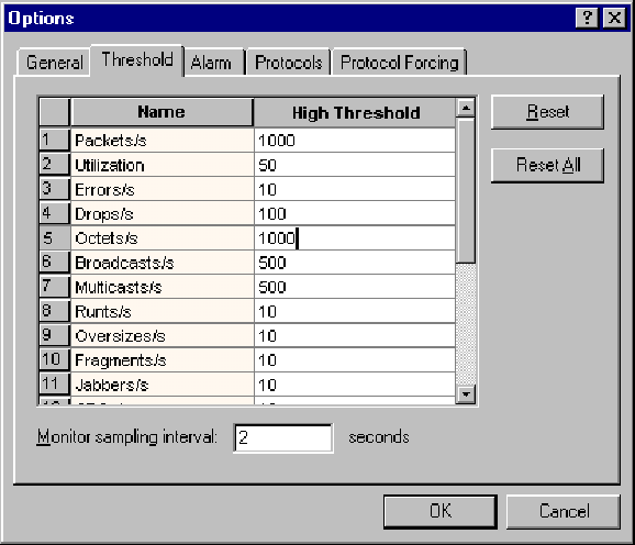
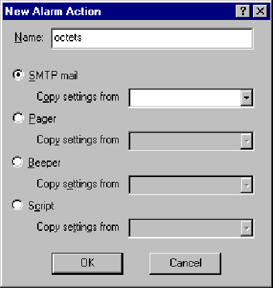
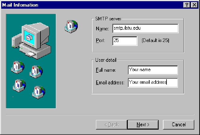
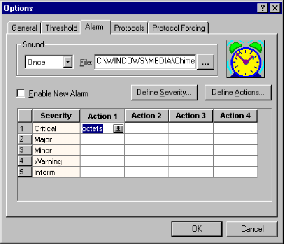
From: ...
Subject: Octets/s: current value = 22086, High Threshold = 9000 To: ...
This event occurred on ...
Save the following files:
-
The “Baseline screens”
-
The Baseline Multiple History.csv file
-
The “alarm e-mail”.
14.9-5 The goal of this practice is to build and validate a baseline model using a network modelling tool. It's supposed that a modelling tool such as COMNET or OPNET is available for the modeller.
First collect response time statistics by pinging a remote computer. The ping command measures the time required for a packet to take a round trip between the client and the server. A possible format of the command is the following: ping hostname -n x -l y -w z > filename where “x” is the number of packet to be sent, “y” is the packet length in bytes, “z” is the time value and “filename” is the name of the file that includes the collected statistics.
For example the ping 138.87.169.13 -n 5 -l 64 > c:
ping.txt command results the following file:
Pinging 138.87.169.13 with 64 bytes of data:
Reply from 138.87.169.13: bytes=64 time=178ms TTL=124
Reply from 138.87.169.13: bytes=64 time=133ms TTL=124
Reply from 138.87.169.13: bytes=64 time=130ms TTL=124
Reply from 138.87.169.13: bytes=64 time=127ms TTL=124
Reply from 138.87.169.13: bytes=64 time=127ms TTL=124
-
Create a histogram for these time values and the sequence number of the packets by using a spreadsheet manager.
-
Create a histogram about the number of responses and the response times.
-
Create the cumulative density function of the response times indicating the details at the tail of the distribution.
-
Create the baseline model of the transfers. Define the traffic attributes by the density function created in the previous step.
-
Validate the model.
-
How much is the link utilization in case of messages with length of 32 and 64 bytes?
14.9-6 It is supposed that a modelling tool (e.g., COMNET, OPNET, etc.) is available for the modeller. In this practice we intend to determine the place of some frequently accessed image file in a lab. The prognosis says that the addition of clients next year will triple the usage of these image files. These files can be stored on the server or on the client workstation. We prefer storing them on a server for easier administration. We will create a baseline model of the current network, we measure the link-utilization caused by the file transfers. Furthermore we validate the model with the correct traffic attributes. By scaling the traffic we can create a forecast about the link- utilization in case of trippled traffic after the addition of the new clients.
-
Create the topology of the baseline model.
-
Capture traffic trace information during the transfer and import them.
-
Run and validate the model (The number of transferred messages in the model must be equal to the number in the trace file, the time of simulation must be equal to the sum of the Interpacket Times and the link utilization must be equal to the average utilization during capture).
-
Print reports about the number of transferred messages, the message delays, the link utilization of the protocols and the total utilization of the link.
-
Let's triple the traffic.
-
Print reports about the number of transferred messages, the message delay, the link utilization of the protocols and the total utilization of the link.
-
If the link-utilization is under the baseline threshold then we leave the images on the server otherwise we move them to the workstations.
-
What is your recommendation: Where is better place to store the image files, the client or the server?
14.9-7 The aim of this practice to compare the performance of the shared and the switched Ethernet. It can be shown that transformation of the shared Ethernet to switched one is only reasonable if the number of collisions exceeds a given threshold.
a. Create the model of a client/server application that uses shared Ethernet LAN. The model includes 10Base5 Ethernet that connects one Web server and three group of workstations. Each group has three PCs, furthermore each group has a source that generates “Web Request” messages. The Web server application of the server responds to them. Each “Web Request” generates traffic toward the server. When the “Web Request” message is received by the server a “Web Response” message is generated and sent to the appropriate client.
-
Each “Web Request” means a message with 10,000 bytes of length sent by the source to the Web Server every Exp(5) second. Set the text of the message to “Web Request”.
-
The Web server sends back a message with the “Web Response” text. The size of the message varies between 10,000 and 100,000 bytes that determined by the Geo(10000, 100000) distribution. The server responds only to the received “Web Request” messages. Set the reply message to “Web Response”.
-
For the rest of the parameters use the default values.
-
Select the “Channel Utilization” and the (“Collision Stats”) at the (“Links Repor”).
-
Select the “Message Delay” at the (“Message + Response Source Report”).
-
Run the simulation for 100 seconds. Animation option can be set.
-
Print the report that shows the “Link Utilization”, the “Collision Statistics” and the report about the message delays between the sources of the traffic.
b. In order to reduce the response time transform the shared LAN to switched LAN. By keeping the clien/server parameters unchanged, deploy an Ethernet switch between the clients and the server. (The server is connected to the switch with full duplex 10Base5 connection.)
-
Print the report of “Link Utilization” and “Collision Statistics”, furthermore the report about the message delays between the sources of the traffic.
c. For all of the two models change the 10Base5 connections to 10BaseT. Unlike the previous situations we will experience a non-equivalent improvement of the response times. We have to give explanation.
14.9-8 A part of a corporate LAN consists of two subnets. Each of them serves a department. One operates according to IEEE 802.3 CSMA/CD 10BaseT Ethernet standard, while the other communicates with IEEE 802.5 16Mbps Token Ring standard. The two subnets are connected with a Cisco 2500 series router. The Ethernet LAN includes 10 PCs, one of them functions as a dedicated mail server for all the two departments. The Token Ring LAN includes 10 PC's as well, one of them operates as a file server for the departments.
The corporation plans to engage employees for both departments. Although the current network configuration won't be able to serve the new employees, the corporation has no method to measure the network utilization and its latency. Before engaging the new employees the corporation would like to estimate these current baseline levels. Employees have already complained about the slowness of download from the file server.
According to a survey, most of the shared traffic flown through the LAN originates from the following sources: electronic mailing, file transfers of applications and voice based messaging systems (Leaders can send voice messages to their employees). The conversations with the employees and the estimate of the average size of the messages provides the base for the statistical description of the message parameters.
E-mailing is used by all employees in both departments. The interviews revealed that the time interval of the mail sending can be characterised with an Exponential distribution. The size of the mails can be described with an Uniform distribution accordingly the mail size is between 500 and 2,000 bytes. All of the emails are transferred to the email server located in the Ethernet LAN, where they are be stored in the appropriate user's mailbox.
The users are able to read messages by requesting them from the email server. The checking of the mailbox can be characterised with a Poisson distribution whose mean value is 900 seconds. The size of the messages used for this transaction is 60 bytes. When a user wants to download an email, the server reads the mailbox file that belongs to the user and transfers the requested mail to the user's PC. The time required to read the files and to process the messages inside can be described with an Uniform distribution that gathers its value from the interval of 3 and 5 seconds. The size of the mails can be described with a normal distribution whose mean value is 40,000 bytes and standard deviation is 10,000 bytes.
Both departments have 8 employees, each of them has their own computer, furthermore they download files from the file server. Arrival interval of these requests can be described as an Exponential distribution with a mean value of 900 ms. The requests' size follows Uniform distribution, with a minimum of 10 bytes minimum and a maximum of 20 bytes. The requests are only sent to the file server located in the Token Ring network. When a request arrives to the server, it read the requested file and send to the PC. This processing results in a very low latency. The size of the files can be described with a normal distribution whose mean value is 20,000 bytes and standard deviation is 25,000 bytes.
Voice-based messaging used only by the heads of the two departments, sending such messages only to theirs employees located in the same department. The sender application makes connection to the employee's PC. After successful connection the message will be transferred. The size of these messages can be described by normal distribution with a mean value of 50,000 bytes and a standard deviation of 1,200 bytes. Arrival interval can be described with a Normal distribution whose mean value is 1,000 seconds and standard deviation is 10 bytes.
TCP/IP is used by all message sources, and the estimated time of packet construction is 0.01 ms.
The topology of the network must be similar to the one in COMNET, Figure 14.50.
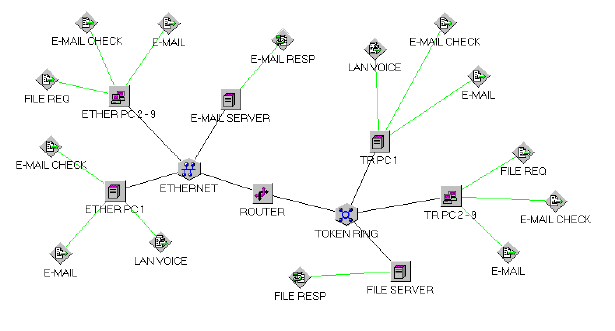
The following reports can be used for the simulation:
-
Link Reports: Channel Utilization and Collision Statistics for each link.
-
Node Reports: Number of incoming messages for the node.
-
Message and Response Reports: The delay of the messages for each node.
-
Session Source Reports: Message delay for each node.
By running the model, a much higher response time will be observed at the file server. What type of solution can be proposed to reduce the response time when the quality of service level requires a lower response time? Is it a good idea to set up a second file server on the LAN? What else can be modified?
CHAPTER NOTES |
Law and Kelton's monography [217] provides a good overview about the network systems e.g. we definition of the networks in Section 14.1 is taken from it. About the classification of computer networks we propose two monography, whose authors are Sima, Fountain és Kacsuk [304], and Tanenbaum [313].
Concerning the basis of probability the book of Alfréd, Rényi [286] is recommended. We have summarised the most common statistical distribution by the book of Banks et al. [29]. The review of COMNET simulation modelling tool used to depict the density functions can be found in two publications of CACI (Consolidated Analysis Centers, Inc.) [53], [186].
Concerning the background of mathematical simulation the monography of Ross [291], and concerning the queueing theory the book of Kleinrock [200] are useful.
The definition of channel capacity can be found in the dictionaries that are available on the Internet [173], [340]. Information and code theory related details can be found in Jones and Jones' book [187].
Taqqu and Co. [220], [317] deal with long-range dependency.
Figure 14.1 that describes the estimations of the most common distributions in network modelling is taken from the book of Banks, Carson és Nelson könyvéből [29].
The OPNET software and its documentation can be downloaded from the address found in [259]. Each phase of simulation is discussed fully in this document.
The effect of traffic burstiness is analysed on the basis of Tibor Gyires's and H. Joseph Wenn's articles [151], [152].
Leland and Co., Crovella and Bestavros [77] report measurements about network traffic.
The self-similarity of networks is dealt by Erramilli, Narayan and Willinger [99], Willinger and Co. [344], and Beran [37]. Mandelbrot [234], Paxson és Floyd [267], furthermore the long-range dependent processes was studied by Mandelbrot and van Ness [235].
Traffic routing models can be found in the following publications: [17], [160], [180], [241], [253], [254], [266], [344].
Figure 14.22 is from the article of Listanti, Eramo and Sabella [224]. The papers [38], [92], [147], [267] contains data on traffic. Long-range dependency was analysed by Addie, Zukerman and Neame [5], Duffield and O'Connell [91], and Narayan and Willinger [99]. The expression of black box modelling was introduced by Willinger and Paxson [342] in 1997.
Information about the principle of Ockham's Razor can be found on the web page of Francis Heylighen [164]. More information about Sniffer is on Network Associates' web site [239].
Willinger, Taqqu, Sherman and Wilson [343] analyse a structural model. Crovella and Bestavros [77] analysed the traffic of World Wide Web.
The effect of burstiness to network congestion is dealt by Neuts [253], and Molnár, Vidács, and Nilsson [248].
The pareto-model and the effect of the Hurst parameter is studied by Addie, Zukerman and Neame [5]. The Benoit-package can be downloaded from the Internet [326].
Table of Contents
Parallel computations is concerned with solving a problem faster by using multiple processors in parallel. These processors may belong to a single machine, or to different machines that communicate through a network. In either case, the use of parallelism requires to split the problem into tasks that can be solved simultaneously.
In the following, we will take a brief look at the history of parallel computing, and then discuss reasons why parallel computing is harder than sequential computing. We explain differences from the related subjects of distributed and concurrent computing, and mention typical application areas. Finally, we outline the rest of this chapter.
Although the history of parallel computing can be followed back even longer, the first parallel computer is commonly said to be Illiac IV, an experimental 64-processor machine that became operational in 1972. The parallel computing area boomed in the late 80s and early 90s when several new companies were founded to build parallel machines of various types. Unfortunately, software was difficult to develop and non-portable at that time. Therefore, the machines were only adopted in the most compute-intensive areas of science and engineering, a market too small to commence for the high development costs. Thus many of the companies had to give up.
On the positive side, people soon discovered that cheap parallel computers can be built by interconnecting standard PCs and workstations. As networks became faster, these so-called clusters soon achieved speeds of the same order as the special-purpose machines. At present, the Top 500 list, a regularly updated survey of the most powerful computers worldwide, contains 42% clusters. Parallel computing also profits from the increasing use of multiprocessor machines which, while designed as servers for web etc., can as well be deployed in parallel computing. Finally, software portability problems have been solved by establishing widely used standards for parallel programming. The most important standards, MPI and OpenMP, will be explained in Subsections 15.3.1 and 15.3.2 of this book.
In summary, there is now an affordable hardware basis for parallel computing. Nevertheless, the area has not yet entered the mainstream, which is largely due to difficulties in developing parallel software. Whereas writing a sequential program requires to find an algorithm, that is, a sequence of elementary operations that solves the problem, and to formulate the algorithm in a programming language, parallel computing poses additional challenges:
-
Elementary operations must be grouped into tasks that can be solved concurrently.
-
The tasks must be scheduled onto processors.
-
Depending on the architecture, data must be distributed to memory modules.
-
Processes and threads must be managed, i.e., started, stopped and so on.
-
Communication and synchronisation must be organised.
Of course, it is not sufficient to find any grouping, schedule etc. that work, but it is necessary to find solutions that lead to fast programs. Performance measures and general approaches to performance optimisation will be discussed in Section 15.2, where we will also elaborate on the items above. Unlike in sequential computing, different parallel architectures and programming models favour different algorithms.
In consequence, the design of parallel algorithms is more complex than the design of sequential algorithms. To cope with this complexity, algorithm designers often use simplified models. For instance, the Parallel Random Access Machine (see Subsection 15.4.1) provides a model in which opportunities and limitations of parallelisation can be studied, but it ignores communication and synchronisation costs.
We will now contrast parallel computing with the related fields of distributed and concurrent computing. Like parallel computing, distributed computing uses interconnected processors and divides a problem into tasks, but the purpose of division is different. Whereas in parallel computing, tasks are executed at the same time, in distributed computing tasks are executed at different locations, using different resources. These goals overlap, and many applications can be classified as both parallel and distributed, but the focus is different. Parallel computing emphasises homogeneous architectures, and aims at speeding up applications, whereas distributed computing deals with heterogeneity and openness, so that applications profit from the inclusion of different kinds of resources. Parallel applications are typically stand-alone and predictable, whereas distributed applications consist of components that are brought together at runtime.
Concurrent computing is not bound to the existence of multiple processors, but emphasises the fact that several sub-computations are in progress at the same time. The most important issue is guaranteeing correctness for any execution order, which can be parallel or interleaved. Thus, the relation between concurrency and parallelism is comparable to the situation of reading several books at a time. Reading the books concurrently corresponds to having a bookmark in each of them and to keep track of all stories while switching between books. Reading the books in parallel, in contrast, requires to look into all books at the same time (which is probably impossible in practice). Thus, a concurrent computation may or may not be parallel, but a parallel computation is almost always concurrent. An exception is data parallelism, in which the instructions of a single program are applied to different data in parallel. This approach is followed by SIMD architectures, as described below.
For the emphasis on speed, typical application areas of parallel computing are science and engineering, especially numerical solvers and simulations. These applications tend to have high and increasing computational demands, since more computing power allows one to work with more detailed models that yield more accurate results. A second reason for using parallel machines is their higher memory capacity, due to which more data fit into a fast memory level such as cache.
The rest of this chapter is organised as follows: In Section 15.1, we give a brief overview and classification of current parallel architectures. Then, we introduce basic concepts such as task and process, and discuss performance measures and general approaches to the improvement of efficiency in Section 15.2. Next, Section 15.3 describes parallel programming models, with focus on the popular MPI and OpenMP standards. After having given this general background, the rest of the chapter delves into the subject of parallel algorithms from a more theoretical perspective. Based on example algorithms, techniques for parallel algorithm design are introduced. Unlike in sequential computing, there is no universally accepted model for parallel algorithm design and analysis, but various models are used depending on purpose. Each of the models represents a different compromise between the conflicting goals of accurately reflecting the structure of real architectures on one hand, and keeping algorithm design and analysis simple on the other. Section 15.4 gives an overview of the models, Section 15.5 introduces the basic concepts of parallel algorithmics, Sections 15.6 and 15.7 explain deterministic example algorithms for PRAM and mesh computational model.
A simple, but well-known classification of parallel architectures has been given in 1972 by Michael Flynn. He distinguishes computers into four classes: SISD, SIMD, MISD, and MIMD architectures, as follows:
-
SI stands for “single instruction”, that is, the machine carries out a single instruction at a time.
-
MI stands for “multiple instruction”, that is, different processors may carry out different instructions at a time.
-
SD stands for “single data”, that is, only one data item is processed at a time.
-
MD stands for “multiple data”, that is, multiple data items may be processed at a time.
SISD computers are von-Neumann machines. MISD computers have probably never been built. Early parallel computers were SIMD, but today most parallel computers are MIMD. Although the scheme is of limited classification power, the abbreviations are widely used.
The following more detailed classification distinguishes parallel machines into SIMD, SMP, ccNUMA, nccNUMA, NORMA, clusters, and grids.
As depicted in Figure 15.1, a SIMD computer is composed of a powerful control processor and several less powerful processing elements (PEs). The PEs are typically arranged as a mesh so that each PE can communicate with its immediate neighbours. A program is a single thread of instructions. The control processor, like the processor of a sequential machine, repeatedly reads a next instruction and decodes it. If the instruction is sequential, the control processor carries out the instruction on data in its own memory. If the instruction is parallel, the control processor broadcasts the instruction to the various PEs, and these simultaneously apply the instruction to different data in their respective memories. As an example, let the instruction be LD reg, 100. Then, all processors load the contents of memory address 100 to reg, but memory address 100 is physically different for each of them. Thus, all processors carry out the same instruction, but read different values (therefore “SIMD”). For a statement of the form if test then if_branch else else_branch, first all processors carry out the test simultaneously, then some carry out if_branch while the rest sits idle, and finally the rest carries out else_branch while the formers sit idle. In consequence, SIMD computers are only suited for applications with a regular structure. The architectures have been important historically, but nowadays have almost disappeared.
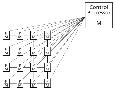
Symmetric multiprocessors (SMP) contain multiple processors that are connected to a single memory. Each processor may access each memory location through standard load/store operations of the hardware. Therefore, programs, including the operating system, must only be stored once. The memory can be physically divided into modules, but the access time is the same for each pair of a processor and a memory module (therefore “symmetric”). The processors are connected to the memory by a bus (see Figure 15.2), by a crossbar, or by a network of switches. In either case, there is a delay for memory accesses which, partially due to competition for network resources, grows with the number of processors.
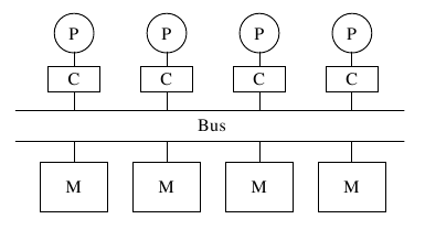
In addition to main memory, each processor has one or several levels of cache with faster access. Between memory and cache, data are moved in units of cache lines. Storing a data item in multiple caches (and writing to it) gives rise to coherency problems. In particular, we speak of false sharing if several processors access the same cache line, but use different portions of it. Since coherency mechanisms work at the granularity of cache lines, each processor assumes that the other would have updated its data, and therefore the cache line is sent back and forth.
NUMA stands for Non-Uniform Memory Access, and contrasts with the symmetry property of the previous class. The general structure of ccNUMA architectures is depicted in Figure 15.3.
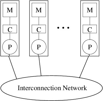
As shown in the figure, each processor owns a local memory, which can be accessed faster than the rest called remote memory. All memory is accessed through standard load/store operations, and hence programs, including the operating system, must only be stored once. As in SMPs, each processor owns one or several levels of cache; cache coherency is taken care of by the hardware.
nccNUMA (non cache coherent Non-Uniform Memory Access) architectures differ from ccNUMA architectures in that the hardware puts into a processor's cache only data from local memory. Access to remote memory can still be accomplished through standard load/store operations, but it is now up to the operating system to first move the corresponding page to local memory. This difference simplifies hardware design, and thus nccNUMA machines scale to higher processor numbers. On the backside, the operating system gets more complicated, and the access time to remote memory grows. The overall structure of Figure 15.3 applies to nccNUMA architectures as well.
NORMA (NO Remote Memory Acess) architectures differ from the previous class in that the remote memory must be accessed through slower I/O operations as opposed to load/store operations. Each node, consisting of processor, cache and local memory, as depicted in Figure 15.3, holds an own copy of the operating system, or at least of central parts thereof. Whereas SMP, ccNUMA, and nccNUMA architectures are commonly classified as shared memory machines, SIMD architectures, NORMA architectures, clusters, and grids (see below) fall under the heading of distributed memory.
According to Pfister, a cluster is a type of parallel or distributed system that consists of a collection of interconnected whole computers that are used as a single, unified computing resource. Here, the term “whole computer” denotes a PC, workstation or, increasingly important, SMP, that is, a node that consists of processor(s), memory, possibly peripheries, and operating system. The use as a single, unified computing resource is also denoted as single system image SSI. For instance, we speak of SSI if it is possible to login into the system instead of into individual nodes, or if there is a single file system. Obviously, the SSI property is gradual, and hence the borderline to distributed systems is fuzzy. The borderline to NORMA architectures is fuzzy as well, where the classification depends on the degree to which the system is designed as a whole instead of built from individual components.
Clusters can be classified according to their use for parallel computing, high throughput computing, or high availability. Parallel computing clusters can be further divided into dedicated clusters, which are solely built for the use as parallel machines, and campus-wide clusters, which are distributed systems with part-time use as a cluster. Dedicated clusters typically do not contain peripheries in their nodes, and are interconnected through a high-speed network. Nodes of campus-wide clusters, in contrast, are often desktop PCs, and the standard network is used for intra-cluster communication.
A grid is a hardware/software infrastructure for shared usage of resources and problem solution. Grids enable coordinated access to resources such as processors, memories, data, devices, and so on. Parallel computing is one out of several emerging application areas. Grids differ from other parallel architectures in that they are large, heterogeneous, and dynamic. Management is complicated by the fact that grids cross organisational boundaries.
As explained in the introduction, parallel computing splits a problem into tasks that are solved independently. The tasks are implemented as either processes or threads. A detailed discussion of these concepts can be found in operating system textbooks such as Tanenbaum. Briefly stated, processes are programs in execution. For each process, information about resources such as memory segments, files, and signals is stored, whereas threads exist within processes such that multiple threads share resources. In particular, threads of a process have access to shared memory, while processes (usually) communicate through explicit message exchange. Each thread owns a separate PC and other register values, as well as a stack for local variables. Processes can be considered as units for resource usage, whereas threads are units for execution on the CPU. As less information needs to be stored, it is faster to create, destroy and switch between threads than it is for processes.
Whether threads or processes are used, depends on the architecture. On shared-memory machines, threads are usually faster, although processes may be used for program portability. On distributed memory machines, only processes are a priori available. Threads can be used if there is a software layer (distributed shared memory) that implements a shared memory abstraction, but these threads have higher communication costs.
Whereas the notion of tasks is problem-related, the notions of processes and threads refer to implementation. When designing an algorithm, one typically identifies a large number of tasks that can potentially be run in parallel, and then maps several of them onto the same process or thread.
Parallel programs can be written in two styles that can also be mixed: With data parallelism, the same operation is applied to different data at a time. The operation may be a machine instruction, as in SIMD architectures, or a complex operation such as a function application. In the latter case, different processors carry out different instructions at a time. With task parallelism, in contrast, the processes/threads carry out different tasks. Since a function may have an if or case statement as the outermost construct, the borderline between data parallelism and task parallelism is fuzzy.
Parallel programs that are implemented with processes can be further classified as using Single Program Multiple Data (SPMD) or Multiple Program Multiple Data (MPMD) coding styles. With SPMD, all processes run the same program, whereas with MPMD they run different programs. MPMD programs are task-parallel, whereas SPMD programs may be either task-parallel or data-parallel. In SPMD mode, task parallelism is expressed through conditional statements.
As the central goal of parallel computing is to run programs faster, performance measures play an important role in the field. An obvious measure is execution time, yet more frequently the derived measure of speedup is used. For a given problem, speedup is defined by
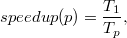
where  denotes the running time of the fastest sequential algorithm, and
  denotes the running time of the parallel algorithm on
  processors. Depending on context, speedup may alternatively refer to using
  processes or threads instead of
  processors. A related, but less frequently used measure is efficiency, defined by
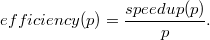
Unrelated to this definition, the term efficiency is also used informally as a synonym for good performance.
Figure 15.4 shows ideal, typical, and super-linear speedup curves. The ideal curve reflects the assumption that an execution that uses twice as many processors requires half of the time. Hence, ideal speedup corresponds to an efficiency of one. Super-linear speedup may arise due to cache effects, that is, the use of multiple processors increases the total cache size, and thus more data accesses can be served from cache instead of from slower main memory.
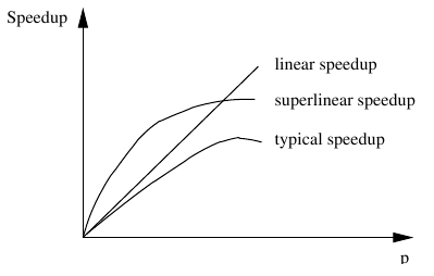
Typical speedup stays below ideal speedup, and grows up to some number of processors. Beyond that, use of more processors slows down the program. The difference between typical and ideal speedups has several reasons:
-
Amdahl's law states that each program contains a serial portion
 that is not amenable to parallelisation. Hence,
  , and thus
  , that is, the speedup is bounded from above by a constant. Fortunately, another observation, called Gustafson-Barsis law reduces the practical impact of Amdahl's law. It states that in typical applications, the parallel variant does not speed up a fixed problem, but runs larger instances thereof. In this case,
  may grow slower than
  , so that
  is no longer constant.
 -
Task management, that is, the starting, stopping, interrupting and scheduling of processes and threads, induces a certain overhead. Moreover, it is usually impossible, to evenly balance the load among the processes/threads.
-
Communication and synchronisation slow down the program. Communication denotes the exchange of data, and synchronisation denotes other types of coordination such as the guarantee of mutual exclusion. Even with high-speed networks, communication and synchronisation costs are orders of magnitude higher than computation costs. Apart from physical transmission costs, this is due to protocol overhead and delays from competition for network resources.
Performance can be improved by minimising the impact of the factors listed above. Amdahl's law is hard to circumvent, except that a different algorithm with smaller  may be devised, possibly at the price of larger
  . Algorithmic techniques will be covered in later sections; for the moment, we concentrate on the other performance factors.
As explained in the previous section, tasks are implemented as processes or threads such that a process/thread typically carries out multiple tasks. For high performance, the granularity of processes/threads should be chosen in relation to the architecture. Too many processes/threads unnecessarily increase the costs of task management, whereas too few processes/threads lead to poor machine usage. It is useful to map several processes/threads onto the same processor, since the processor can switch when it has to wait for I/O or other delays. Large-granularity processes/threads have the additional advantage of a better communication-to-computation ratio, whereas fine-granularity processes/threads are more amenable to load balancing.
Load balancing can be accomplished with static or dynamic schemes. If the running time of the tasks can be estimated in advance, static schemes are preferable. In these schemes, the programmer assigns to each process/thread some number of tasks with about the same total costs. An example of a dynamic scheme is master/slave. In this scheme, first a master process assigns one task to each slave process. Then, repeatedly, whenever a slave finishes a task, it reports to the master and is assigned a next task, until all tasks have been processed. This scheme achieves good load balancing at the price of overhead for task management.
The highest impact on performance usually comes from reducing communication/synchronisation costs. Obvious improvements result from changes in the architecture or system software, in particular from reducing latency, that is, the delay for accessing a remote data item, and bandwidth, that is, the amount of data that can be transferred per unit of time.
The algorithm designer or application programmer can reduce communication/synchronisation costs by minimising the number of interactions. An important approach to achieve this minimisation is locality optimisation. Locality, a property of (sequential or parallel) programs, reflects the degree of temporal and spatial concentration of accesses to the same data. In distributed-memory architectures, for instance, data should be stored at the processor that uses the data. Locality can be improved by code transformations, data transformations, or a combination thereof. As an example, consider the following program fragment to be executed on three processors:
       for (i=0; i<N; i++) in parallel
          for (j=0; j<N; j++)
             f(A[i][j]);
Here, the keyword “in parallel” means that the iterations are evenly distributed among the processors so that  runs iterations
 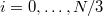 ,
,  runs iterations
  , and
, and  runs iterations
  (rounded if necessary). The function
  is supposed to be free of side effects.
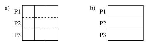
With the data distribution of Figure 15.5a), locality is poor, since many accesses refer to remote memory. Locality can be improved by changing the data distribution to that of Figure 15.5b) or, alternatively, by changing the program into
       for (j=0; j<N; j++) in parallel
          for (i=0; i<N; i++)
             f(A[i][j]);
The second alternative, code transformations, has the advantage of being applicable selectively to a portion of code, whereas data transformations influence the whole program so that an improvement in one part may slow down another. Data distributions are always correct, whereas code transformations must respect data dependencies, which are ordering constraints between statements. For instance, in
       a = 3; (1)
       b = a; (2)
a data dependence occurs between statements (1) and (2). Exchanging the statements would lead to an incorrect program.
On shared-memory architectures, a programmer does not the specify data distribution, but locality has a high impact on performance, as well. Programs run faster if data that are used together are stored in the same cache line. On shared-memory architectures, the data layout is chosen by the compiler, e.g. row-wise in C. The programmer has only indirect influence through the manner in which he or she declares data structures.
Another opportunity to reduce communication costs is replication. For instance, it pays off to store frequently used data at multiple processors, or to repeat short computations instead of communicating the result.
Synchronisations are necessary for correctness, but they slow down program execution, first because of their own execution costs, and second because they cause processes to wait for each other. Therefore, excessive use of synchronisation should be avoided. In particular, critical sections (in which processes/threads require exclusive access to some resource) should be kept at a minimum. We speak of sequentialisation if only one process is active at a time while the others are waiting.
Finally, performance can be improved by latency hiding, that is, parallelism between computation and communication. For instance, a process can start a remote read some time before it needs the result (prefetching), or write data to remote memory in parallel to the following computations.
Exercises
15.2-1 For standard matrix multiplication, identify tasks that can be solved in parallel. Try to identify as many tasks as possible. Then, suggest different opportunities for mapping the tasks onto (a smaller number of) threads, and compare these mappings with respect to their efficiency on a shared-memory architecture.
15.2-2 Consider a parallel program that takes as input a number  and computes as output the number of primes in range
  . Task
  of the program should determine whether
  is a prime, by systematically trying out all potential factors, that is, dividing by
  . The program is to be implemented with a fixed number of processes or threads. Suggest different opportunities for this implementation and discuss their pros and cons. Take into account both static and dynamic load balancing schemes.
15.2-3 Determine the data dependencies of the following stencil code:
       for (t=0; t<tmax; t++)
          for (i=0; i<n; i++)
             for (j=0; j<n; j++)
                a[i][j] += a[i-1][j] + a[i][j-1]
Restructure the code so that it can be parallelised.
15.2-4 Formulate and prove the bounds of the speedup known as Amdahl law and Gustafson-Barsis law. Explain the virtual contradiction between these laws. What can you say on the practical speedup?
Partly due to the use of different architectures and the novelty of the field, a large number of parallel programming models has been proposed. The most popular models today are message passing as specified in the Message Passing Interface standard (MPI), and structured shared-memory programming as specified in the OpenMP standard. These programming models are discussed in Subsections 15.3.1 and 15.3.2, respectively. Other important models such as threads programming, data parallelism, and automatic parallelisation are outlined in Subsection 15.3.3.
As the name says, MPI is based on the programming model of message passing. In this model, several processes run in parallel and communicate with each other by sending and receiving messages. The processes do not have access to a shared memory, but accomplish all communication through explicit message exchange. A communication involves exactly two processes: one that executes a send operation, and another that executes a receive operation. Beyond message passing, MPI includes collective operations and other communication mechanisms.
Message passing is asymmetric in that the sender must state the identity of the receiver, whereas the receiver may either state the identity of the sender, or declare its willingness to receive data from any source. As both sender and receiver must actively take part in a communication, the programmer must plan in advance when a particular pair of processes will communicate. Messages can be exchanged for several purposes:
-
exchange of data with details such as the size and types of data having been planned in advance by the programmer
-
exchange of control information that concerns a subsequent message exchange, and
-
synchronisation that is achieved since an incoming message informs the receiver about the sender's progress. Additionally, the sender may be informed about the receiver's progress, as will be seen later. Note that synchronisation is a special case of communication.
The MPI standard has been introduced in 1994 by the MPI forum, a group of hardware and software vendors, research laboratories, and universities. A significantly extended version, MPI-2, appeared in 1997. MPI-2 has about the same core functionality as MPI-1, but introduces additional classes of functions.
MPI describes a set of library functions with language binding to C, C++, and Fortran. With notable exceptions in MPI-2, most MPI functions deal with interprocess communication, leaving issues of process management such as facilities to start and stop processes, open. Such facilities must be added outside the standard, and are consequently not portable. For this and other reasons, MPI programs typically use a fixed set of processes that are started together at the beginning of a program run. Programs can be coded in SPMD or MPMD styles. It is possible to write parallel programs using only six base functions:
-
MPI_Initmust be called before any other MPI function. -
MPI_Finalizemust be called after the last MPI function. -
MPI_Comm_sizeyields the total number of processes in the program. -
MPI_Comm_rankyields the number of the calling process, with processes being numbered starting from 0. -
MPI_Sendsends a message. The function has the following parameters:-
address, size, and data type of the message,
-
number of the receiver,
-
message tag, which is a number that characterises the message in a similar way like the subject characterises an email,
-
communicator, which is a group of processes as explained below.
-
-
MPI_Recvreceives a message. The function has the same parameters as MPI_Send, except that only an upper bound is required for the message size, a wildcard may be used for the sender, and an additional parameter called status returns information about the received message, e.g. sender, size, and tag.
Figure 15.6 depicts an example MPI program.
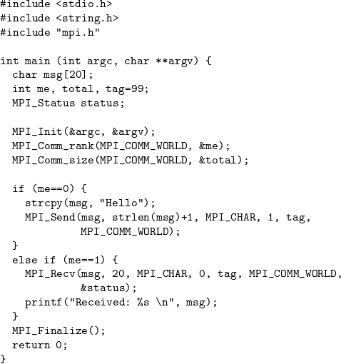
Although the above functions are sufficient to write simple programs, many more functions help to improve the efficiency and/or structure MPI programs. In particular, MPI-1 supports the following classes of functions:
-
Alternative functions for pairwise communication: The base
MPI_Sendfunction, also called standard mode send, returns if either the message has been delivered to the receiver, or the message has been buffered by the system. This decision is left to MPI. Variants ofMPI_Sendenforce one of the alternatives: In synchronous mode, the send function only returns when the receiver has started receiving the message, thus synchronising in both directions. In buffered mode, the system is required to store the message if the receiver has not yet issuedMPI_Recv.On both the sender and receiver sides, the functions for standard, synchronous, and buffered modes each come in blocking and nonblocking variants. Blocking variants have been described above. Nonblocking variants return immediately after having been called, to let the sender/receiver continue with program execution while the system accomplishes communication in the background. Nonblocking communications must be completed by a call to
MPI_WaitorMPI_Testto make sure the communication has finished and the buffer may be reused. Variants of the completion functions allow to wait for multiple outstanding requests.MPI programs can deadlock, for instance if a process
 first issues a send to process
  and then a receive from
  ; and
; and  does the same with respect to
  . As a possible way-out, MPI supports a combined send/receive function.
In many programs, a pair of processes repeatedly exchanges data with the same buffers. To reduce communication overhead in these cases, a kind of address labels can be used, called persistent communication. Finally, MPI functions
MPI_ProbeandMPI_Iprobeallow to first inspect the size and other characteristics of a message before receiving it. -
Functions for Datatype Handling: In simple forms of message passing, an array of equally-typed data (e.g.
float) is exchanged. Beyond that, MPI allows to combine data of different types in a single message, and to send data from non-contiguous buffers such as every second element of an array. For these purposes, MPI defines two alternative classes of functions: user-defined data types describe a pattern of data positions/types, whereas packaging functions help to put several data into a single buffer. MPI supports heterogeneity by automatically converting data if necessary. -
Collective communication functions: These functions support frequent patterns of communication such as broadcast (one process sends a data item to all other processes). Although any pattern can be implemented by a sequence of sends/receives, collective functions should be preferred since they improve program compactness/understandability, and often have an optimised implementation. Moreover, implementations can exploit specifics of an architecture, and so a program that is ported to another machine may run efficiently on the new machine as well, by using the optimised implementation of that machine.
-
Group and communicator management functions: As mentioned above, the send and receive functions contain a communicator argument that describes a group of processes. Technically, a communicator is a distributed data structure that tells each process how to reach the other processes of its group, and contains additional information called attributes. The same group may be described by different communicators. A message exchange only takes place if the communicator arguments of
MPI_SendandMPI_Recvmatch. Hence, the use of communicators partitions the messages of a program into disjoint sets that do not influence each other. This way, communicators help structuring programs, and contribute to correctness. For libraries that are implemented with MPI, communicators allow to separate library traffic from traffic of the application program. Groups/communicators are necessary to express collective communications. The attributes in the data structure may contain application-specific information such as an error handler. In addition to the (intra)communicators described so far, MPI supports intercommunicators for communication between different process groups.MPI-2 adds four major groups of functions:
-
Dynamic process management functions: With these functions, new MPI processes can be started during a program run. Additionally, independently started MPI programs (each consisting of multiple processes) can get into contact with each other through a client/server mechanism.
-
One-sided communication functions: One-sided communication is a type of shared-memory communication in which a group of processes agrees to use part of their private address spaces as a common resource. Communication is accomplished by writing into and reading from that shared memory. One-sided communication differs from other shared-memory programming models such as OpenMP in that explicit function calls are required for the memory access.
-
Parallel I/O functions: A large set of functions allows multiple processes to collectively read from or write to the same file.
-
Collective communication functions for intercommunicators: These functions generalise the concept of collective communication to intercommunicators. For instance, a process of one group may broadcast a message to all processes of another group.
OpenMP derives its name from being an open standard for multiprocessing, that is for architectures with a shared memory. Because of the shared memory, we speak of threads (as opposed to processes) in this section.
Shared-memory communication is fundamentally different from message passing: Whereas message passing immediately involves two processes, shared-memory communication uncouples the processes by inserting a medium in-between. We speak of read/write instead of send/receive, that is, a thread writes into memory, and another thread later reads from it. The threads need not know each other, and a written value may be read by several threads. Reading and writing may be separated by an arbitrary amount of time. Unlike in message passing, synchronisation must be organised explicitly, to let a reader know when the writing has finished, and to avoid concurrent manipulation of the same data by different threads.
OpenMP is one type of shared-memory programming, while others include one-sided communication as outlined in Subsection 15.3.1, and threads programming as outlined in Subsection 15.3.3. OpenMP differs from other models in that it enforces a fork-join structure, which is depicted in Figure 15.7. A program starts execution as a single thread, called master thread, and later creates a team of threads in a so-called parallel region. The master thread is part of the team. Parallel regions may be nested, but the threads of a team must finish together. As shown in the figure, a program may contain several parallel regions in sequence, with possibly different numbers of threads.
As another characteristic, OpenMP uses compiler directives as opposed to library functions. Compiler directives are hints that a compiler may or may not take into account. In particular, a sequential compiler ignores the directives. OpenMP supports incremental parallelisation, in which one starts from a sequential program, inserts directives at the most performance-critical sections of code, later inserts more directives if necessary, and so on.
OpenMP has been introduced in 1998, version 2.0 appeared in 2002. In addition to compiler directives, OpenMP uses a few library functions and environment variables. The standard is available for C, C++, and Fortran.
Programming OpenMP is easier than programming MPI since the compiler does part of the work. An OpenMP programmer chooses the number of threads, and then specifies work sharing in one of the following ways:
-
Explicitly: A thread can request its own number by calling the library function
omp_get_thread_num. Then, a conditional statement evaluating this number explicitly assigns tasks to the threads, similar as in SPMD-style MPI programs. -
Parallel loop: The compiler directive
#pragma omp parallel forindicates that the followingforloop may be executed in parallel so that each thread carries out several iterations (tasks). An example is given in Figure 15.8. The programmer can influence the work sharing by specifying parameters such asschedule(static)orschedule(dynamic). Static scheduling means that each thread gets an about equal-sized block of consecutive iterations. Dynamic scheduling means that first each thread is assigned one iteration, and then, repeatedly, a thread that has finished an iteration gets the next one, as in the master/slave paradigma described before for MPI. Different from master/slave, the compiler decides which thread carries out which tasks, and inserts the necessary communications. -
Task-parallel sections: The directive
#pragma omp parallel sectionsallows to specify a list of tasks that are assigned to the available threads.
Threads communicate through shared memory, that is, they write to or read from shared variables. Only part of the variables are shared, while others are private to a particular thread. Whether a variable is private or shared is determined by rules that the programmer can overwrite.
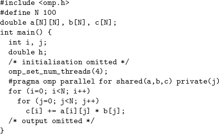
Many OpenMP directives deal with synchronisation that is necessary for mutual exclusion, and to provide a consistent view of shared memory. Some synchronisations are inserted implicitly by the compiler. For instance, at the end of a parallel loop all threads wait for each other before proceeding with a next loop.
While MPI and OpenMP are the most popular models, other approaches have practical importance as well. Here, we outline threads programming, High Performance Fortran, and automatic parallelisation.
Like OpenMP, threads programming or by Java threads uses shared memory. Threads operate on a lower abstraction level than OpenMP in that the programmer is responsible for all details of thread management and work sharing. In particular, threads are created explicitly, one at a time, and each thread is assigned a function to be carried out. Threads programming focuses on task parallelism, whereas OpenMP programming focuses on data parallelism. Thread programs may be unstructured, that is, any thread may create and stop any other. OpenMP programs are often compiled into thread programs.
Data parallelism provides for a different programming style that is explicitly supported by languages such as High Performance Fortran (HPF). While data parallelism can be expressed in MPI, OpenMP etc., data-parallel languages center on the approach. As one of its major constructs, HPF has a parallel loop whose iterations are carried out independently, that is, without communication. The data-parallel style makes programs easier to understand since there is no need to take care of concurrent activities. On the backside, it may be difficult to force applications into this structure. HPF is targeted at single address space distributed memory architectures, and much of the language deals with expressing data distributions. Whereas MPI programmers distribute data by explicitly sending them to the right place, HPF programmers specify the data distribution on a similar level of abstraction as OpenMP programmers specify the scheduling of parallel loops. Details are left to the compiler. An important concept of OpenMP is the owner-computes rule, according to which the owner of the left-hand side variable of an assignment carries out an operation. Thus, data distribution implies the distribution of computations.
Especially for programs from scientific computing, a significant performance potential comes from parallelising loops. This parallelisation can often be accomplished automatically, by parallelising compilers. In particular, these compilers check for data dependencies. that prevent parallelisation. Many programs can be restructured to circumvent the dependence, for instance by exchanging outer and inner loops. Parallelising compilers find these restructuring for important classes of programs.
Exercises
15.3-1 Sketch an MPI program for the prime number problem of Exercise 15.2-3. The program should deploy the master/slave paradigma. Does your program use SPMD style or MPMD style?
15.3-2 Modify your program from Exercise 15.3-1 so that it uses collective communication.
15.3-3 Compare MPI and OpenMP with respect to programmability, that is, give arguments why or to which extent it is easier to program in either MPI or OpenMP.
15.3-4 Sketch an OpenMP program that implements the stencil code example of Exercise 15.2-3.
The most popular computational model is the Parallel Random Access Machine (PRAM) which is a natural generalisation of the Random Access Machine (RAM).
The PRAM model consists of  synchronised processors
  , a shared memory with memory cells
  and memories of the processors. Figure 15.9. shows processors and the shared random access memory
There are variants of this model. They differ in whether multiple processors are allowed to access the same memory cell in a step, and in how the resulting conflicts are resolved. In particular the following variants are distinguished:
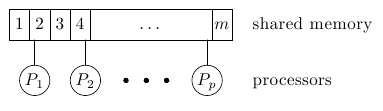
Types on the base of the properties of read/write operations are
-
EREW (Exclusive-Read Exclusive-Write) PRAM,
-
ERCW (Exclusive-Read Concurrent-Write) PRAM,
-
CREW (Concurrent-Read Exclusive-Write) PRAM,
-
CRCW (Concurrent-Read Concurrent-Write) PRAM.
Figure 15.10(a) shows the case when at most one processor has access a memory cell (ER), and Figure 15.10(d) shows, when multiple processors have access the same cell (CW).
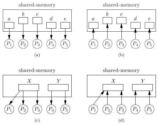
Types of concurrent writing are common, priority, arbitrary, combined.
Here we consider the models BSP, LogP and QSM.
Bulk-synchronous Parallel Model (BSP) describes a computer as a collection of nodes, each consisting of a processor and memory. BSP supposes the existence of a router and a barrier synchronisation facility. The router transfers messages between the nodes, the barrier synchronises all or a subset of nodes. According to BSP computation is partitioned into supersteps. In a superstep each processor independently performs computations on data in its own memory, and initiates communications with other processors. The communication is guaranteed to complete until the beginning of the next superstep.
 is defined such that
  is the time that is takes to route an
  -relation under continuous traffic conditions. An
  -relation is a communication pattern in which each processor sends and receives up to
  messages.
The cost of a superstep is determined as  , where
  is the maximum number of communications initiated by any processor. The cost of a program is the sum of the costs of the individual supersteps.
BSP contains a cost model that involves three parameters: the number of processors  , the cost of a barrier synchronisation
  and a characteristics of the available bandwidth
  .
.
LogP model was motivated by inaccuracies of BSP and the restrictive requirement to follow the superstep structure.
While LogP improves on BSP with respect to reflectivity, QSM improves on it with respect to simplicity. In contrast to BSP, QSM is a shared-memory model. As in BSP, the computation is structured into supersteps, and each processor has its own local memory. In a superstep, a processor performs computations on values in the local memory, and initiates read/write operations to the shared memory. All shared-memory accesses complete until the beginning of the next superstep. QSM allows for concurrent reads and writes. Let the maximum number of accesses to any cell in a superstep be  . Then QSM charges costs
  , with
  , and
, and  being defined in BSP.
Mesh also is a popular computational model. A  -dimensional mesh is an
  sized grid having a processor in each grid point. The edges are the communication lines, working in two directions. Processors are labelled by
  -tuples, as
  .
.
Each processor is a RAM, having a local memory. The local memory of the processor  is
is  . Each processor can execute in one step such basic operations as adding, subtraction, multiplication, division, comparison, read and write from/into the local memory, etc. Processors work in synchronised way, according to a global clock.
The simplest mesh is the chain, belonging to the value  . Figure 15.11 shows a chain consisting of 6 processors.
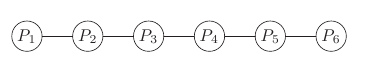
The processors of a chain are  .
.  is connected with
  ,
,  is connected with
  , the remaining processors
  are connected with
  and
and  .
.
If  , then we get a rectangle. If now
  , then we get a square. Figure 15.12 shows a square of size
  .
.
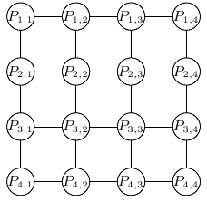
A square contains several chains consisting of  processors. The processors having identical first index, form a row of processors, and the processors having the same second index form a column of processors. Algorithms running on a square often consists of such operations, executed only by processors of some rows or columns.
If  , then the corresponding mesh is a brick. In the special case
 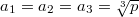 the mesh is called cube. Figure 15.13 shows a cube of size
  .
.
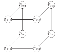
The next model of computation is the d-dimensional hypercube  . This model can be considered as the generalisation of the square and cube: the square represented on Figure 15.12 is a 2-dimensional, and the cube, represented on Figure 15.13 is a 3-dimensional hypercube. The processors of
  can be labelled by a binary number consisting of
  bits. Two processors of
  are connected iff the Hamming-distance of their labels equals to 1. Therefore each processors of
  has
has  neighbours, and the of
  is
is  . Figure 15.14 represents
  .
.
The butterfly model  consists of
  processors and
  edges. The processors can be labelled by a pair
  , where
  is the columnindex and
  is the level of the given processor. Figure 15.15 shows a butterfly model
  containing 32 processors in 8 columns and in 4 levels.
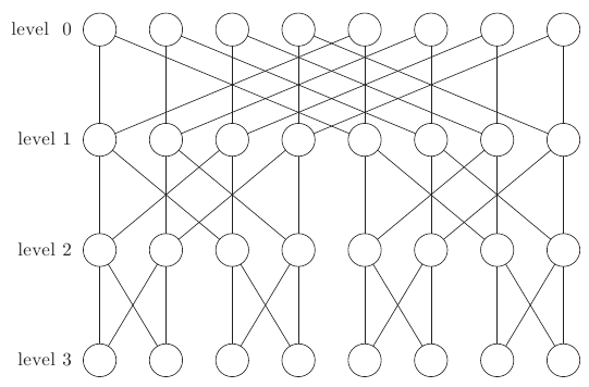
Finally Figure 15.16 shows a ring containing 6 processors.
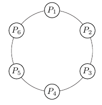
In the previous section we considered the performance measures used in the practice.
In the theoretical investigations the algorithms are tested using abstract computers called computation models.
The required quantity of resources can be characterised using absolute and relative measures.
Let  , resp.
  denote the time necessary in worst case to solve the problem
  of size
  by the sequential algorithm A, resp. parallel algorithm P (using
  processors).
In a similar way let  , resp.
  the time necessary for algorithm A, resp. P in best case to solve the problem
  of size
  (algorithm P can use
  processors).
Let  , resp.
  the time needed by any sequential, resp. parallel algorithm to solve problem
  of size
  (algorithm P can use
  processors). These times represent a lower bound of the corresponding running time.
Let suppose the distribution function  of the problem
  of size
  is given. Then let
  , resp.
  the expected value of the time necessary for algorithm A, resp. P to solve problem
  of size
  (algorithm P uses
  processors).
In the analysis it is often supposed that the input data of equal size have equal probability. For such cases we use the notation  , resp.
  and termin average running time.
The value of the performance measures  and
and  depend on the used computation model too. For the simplicity of notations we suppose that the algorithms determine the computation model.
Usually the context shows in a unique way the investigated problem. If so, then the parameter  is omitted.
Among these performance measures hold the following inequalities:


In a similar way for the characteristic data of the parallel algorithms the following inequalities are true:


For the expected running time we have


and


These notations can be used not only for the running time, but also for any other resource, as memory requirement, number of messages, etc.
Now we define some relative performance measures.
Speedup shows, how many times is smaller the running time of a parallel algorithm, than the running time of the parallel algorithm solving the same problem.
The speedup (or relative number of steps or relative speed) of a given parallel algorithm P, comparing it with a given sequential algorithm A, is defined as

If for a sequential algorithm A and a parallel algorithm P holds

then the speedup of P comparing with A is linear, if

then the speedup of P comparing with A is sublinear, and if

then the speedup of P comparing with A is superlinear.
In the case of parallel algorithms it is a very important performance measure the work  , defined by the product of the running time and the number of the used processors:

This definition is used even then if some processors work only in a small fraction of the running time. Therefore the real work can be much smaller, then given by the formula (15.15).
The efficiency  is a measure of the fraction of time for which the processors are usefully employed; it is defined as the ratio of the work of the sequential algorithm to the work of the parallel algorithm P:

One can observe, that the ratio of the speedup and the number of the used parallel processors results the same value. If the parallel work is not less than the sequential one, then efficiency is between zero and one, and the relatively large values are beneficial.
In connection with the analysis of the parallel algorithms the work-efficiency is a central concept. If for a parallel algorithm P and sequential algorithm A holds

then algorithm P work-optimal comparing with A.
This definition is equivalent with the equality

According to this definition a parallel algorithm is work-optimal only if the order of its total work is not greater, than the order of the total work of the considered sequential algorithm.
A weaker requirement is the following. If there exists a finite positive integer  such that

then algorithm P is work-efficient comparing with A.
If a sequential algorithm A, resp. a parallel algorithm P uses only  , resp.
  units of a given resource, then A, resp. P is called—for the given resource and the considered model of computation—asymptotically optimal.
If an A sequential or a P parallel algorithm uses only the necessary amount of some resource for all possible size  of the input, that is
  , resp.
  units, and so we have

for A and

for P, then we say, that the given algorithm is absolute optimal for the given resource and the given computation model. In this case we say, that  is the accurate complexity of the given problem.
Comparing two algorithms and having

we say, that the speeds of the growths of algorithms  and
and  asymptotically have the same order.
Comparing the running times of two algorithms A and B (e.g. in worst case) sometime the estimation depends on  : for some values of
  algorithm A, while for other values of
  algorithm B is the better. A possible formal definition is as follows. If the functions
  and
and  are defined for all positive integer
  , and for some positive integer
  hold
hold
-
 ;
; -
 ,
,
then the number  is called crossover point of the functions
  and
and  .
.
For example multiplying two matrices according to the definition and algorithm of Strassen we get one crossover point, whose value is about 20.
Exercises
15.5-1 Suppose that the parallel algorithms P and Q solve the selection problem. Algorithm P uses  processors and its running time is
  . Algorithm Q uses
  processors and its running time is
  . Determine the work, speedup and efficiency for both algorithms. Are these algorithms work-optimal or at least work-efficient?
15.5-2 Analyse the following two assertions.
a) Running time of algorithm P is at least  .
.
b) Since the running time of algorithm P is  , and the running time of algorithm B is
  , therefore algorithm B is more efficient.
15.5-3 Extend the definition of the crossover point to noninteger  values and parallel algorithms.
In this section we consider parallel algorithms solving simple problems as prefix calculation, ranking of the elements of an array, merging, selection and sorting.
In the analysis of the algorithms we try to give the accurate order of the running time in the worst case and try to decide whether the presented algorithm is work-optimal or at least work-efficient or not. When parallel algorithms are compared with sequential algorithms, always the best known sequential algorithm is chosen.
To describe these algorithms we use the following pseudocode conventions.

INPARALLEL FOR
TO
DO
. . .

For  PRAM ordered into a square grid of size
  the instruction begin with

IN PARALLEL FOR
TO,

TO
DO
For a  -dimensional mesh of size
  the similar instruction begins with

         IN PARALLEL FOR  TO  TO
             DO
It is allowed that in this commands  represents a group of processors.
Let  be a binary associative operator defined over a set
  . We suppose that the operator needs only one set and the set is closed for this operation.
A binary operation  is associative on a
  set, if for all
  holds
holds

Let the elements of the sequence  be elements of the set
  . Then the input data are the elements of the sequence
  , and the prefix problem is the computation of the elements
  . These elements are called prefixes.
It is worth to remark that in other topics of parallel computations the starting sequences  of the sequence
  are called prefixes.
Example 15.1 Associative operations. If  is the set of integer numbers,
  means addition and the sequence of the input data is
  , then the sequence of the prefixes is
  . If the alphabet and the input data are the same, but the operation is the multiplication, then
  . If the operation is the minimum (it is also an associative operation), then
  . In this case the last prefix is the minimum of the input data.

The prefix problem can be solved by sequential algorithms in  time. Any sequential algorithm A requires
  time to solve the prefix problem. There are parallel algorithms for different models of computation resulting a work-optimal solution of the prefix problem.
In this subsection at first the algorithm CREW-Prefix is introduced, which solves the prefix problem in  time, using
  CREW PRAM processors.
Next is algorithm EREW-Prefix, having similar quantitative characteristics, but requiring only EREW PRAM processors.
These algorithms solve the prefix problem quicker, then the sequential algorithms, but the order of the necessary work is larger.
Therefore interesting is algorithm Optimal-Prefix, which uses only  CREW PRAM processors, and makes only
  steps. The work of this algorithm is only
  , therefore its efficiency is
  , and so it is work-optimal. The speedup of this algorithm equals to
  .
.
For the sake of simplicity in the further we write usually  instead of
  .
.
As first parallel algorithm a recursive algorithm is presented, which runs on CREW PRAM model of computation, uses  processors and
  time. Designing parallel algorithm it is often used the principle divide-and-conquer, as we we will see in the case of the next algorithm too
Input is the number of processors  and the array
  , output data are the array
  . We suppose
  is a power of 2. Since we use the algorithms always with the same number of processors, therefore we omit the number of processors from the list of input parameters. In the mathematical descriptions we prefer to consider
  and
and  as sequences, while in the pseudocodes sometimes as arrays.
CREW-Prefix(
)
1IF2
THEN3
RETURN4
IF5
THEN
INPARALLEL FOR
TO
DOcompute recursive, the prefixes, belonging to

INPARALLEL FOR
TO
DOcompute recursivethe prefixes, belonging to
6

INPARALLEL FOR
DOreadfrom the global memory and compute
7
RETURN
Example 15.2 Calculation of prefixes of 8 elements on 8 processors. Let  and
and  . The input data of the prefix calculation are 12, 3, 6, 8, 11, 4, 5 and 7, the associative operation is the addition.
The run of the recursive algorithm consists of rounds. In the first round (step 4) the first four processors get the input data 12, 3, 6, 8, and compute recursively the prefixes 12, 15, 21, 29 as output. At the same time the other four processors get the input data 11, 4, 5, 7, and compute the prefixes 11, 15, 20, 27.
According to the recursive structure  and
and  work as follows.
  and
and  get
get  and
and  , resp.
  and
and  get
get  and
and  as input. Recursivity mean for
  and
and  , that
  gets
gets  and
and  gets
gets  , computing at first
  and
and  , then
  updates
  . After this
  computes
  and
and  .
.
While  and
and  , according to step 4, compute the final values
  and
and  ,
,  and
and  compute the local provisional values of
  and
and  .
.
In the second round (step 5) the first four processors stay, the second four processors compute the final values of  and
and  , adding
  to the provisional values 11, 15, 20 and 27 and receiving 40, 44, 49 and 56.
In the remaining part of the section we use the notation  instead of
  and give the number of used processors in verbal form. If
  , then we usually prefer to use
  .
.
Theorem 15.1 Algorithm CREW-Prefix uses  time on p
 CREW PRAM processors to compute the prefixes of p elements.
Proof. The lines 4–6 require  steps, the line 7 does
  steps. So we get the following recurrence:

Solution of this recursive equation is  .
.
CREW-prefix is not work-optimal, since its work is  and we know sequential algorithm requiring only
  time, but it is work-effective, since all sequential prefix algorithms require
  time.
time.
In the following algorithm we use exclusive write instead of the parallel one, therefore it can be implemented on the EREW PRAM model. Its input is the number of processors  and the sequence
  , and its output is the sequence
  containing the prefixes.
EREW-Prefix(
)
12

IN PARALLEL FOR
TO3
DO4
5
WHILE6
DO
IN PARALLEL FOR
TO7
DO8
9
RETURN
Theorem 15.2 Algorithm EREW-Prefix computes the prefixes of  elements on
EREW PRAM processors in  time.
time.
Proof. The commands in lines 1–3 and 9 are executed in  time. Lines 4–7 are executed so many times as the assignment in line 8, that is
  times.
Next we consider a recursive work-optimal algorithm, which uses  CREW PRAM processors. Input is the length of the input sequence
  and the sequence
  , output is the sequence
  , containing the computed prefixes.
Optimal-Prefix(
)
1
IN PARALLEL FOR
TO2
DOcompute recursive, the prefixes of the following
input data
3

IN PARALLEL FOR
TO4
DOusingCREW-Prefixcompute, the prefixes of the following
elements:
5

IN PARALLEL FOR
TO6
DOFOR
TO7
DO8

FOR
TO9
DO10
RETURN
This algorithm runs in logarithmic time. The following two formulas help to show it:

and

where summing goes using the corresponding associative operation.
Theorem 15.3 (parallel prefix computation in  time) Algorithm
 Optimal-Prefix computes the prefixes of  elements on
CREW PRAM processors in  time.
time.
Proof. Line 1 runs in  time, line 2 runs
  time, line 3 runs
  time.
time.
This theorem imply that the work of Optimal-Prefix is  , therefore
 Optimal-Prefix is a work-optimal algorithm.
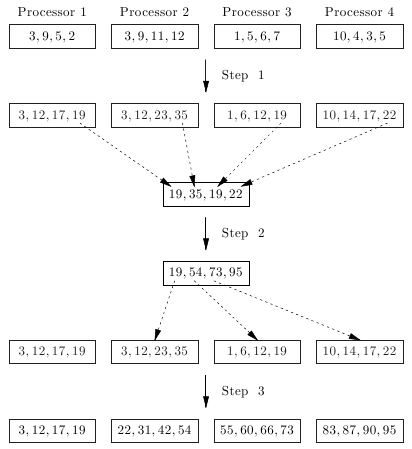
Let the elements of the sequence  be the elements of the alphabet
  . Then the input data of the prefix computation are the elements of the sequence
  , and the prefix problem is the computation of the elements
  . These computable elements are called prefixes.
We remark, that in some books on parallel programming often the elements of the sequence  are called prefixes.
Example 15.3 Associative operations. If  is the set of integers,
  denotes the addition and the sequence of the input data is 3, -5, 8, 2, 5, 4, then the prefixes are 3, -2, 6, 8, 13, 17. If the alphabet and the input data are the same, the operation is the multiplication, then the output data (prefixes) are 3, -15, -120, -240, -1200, -4800. If the operation is the minimum (it is also associative), then the prefixes are 3, -5, -5, -5, -5, -5. The last prefix equals to the smallest input data.
Sequential prefix calculation can be solved in  time. Any A sequential algorithm needs
  time. There exist work-effective parallel algorithms solving the prefix problem.
Our first parallel algorithm is CREW-Prefix, which uses  CREW PRAM processors and requires
  time. Then we continue with algorithm
 EREW-Prefix, having similar qualitative characteristics, but running on EREW PRAM model too.
These algorithms solve the prefix problem quicker, than the sequential algorithms, but the order of their work is larger.
Algorithm Optimal-Prefix requires only  CREW PRAM processors and in spite of the reduced numbers of processors requires only
  time. So its work is
  , therefore its efficiency is
  and is work-effective. The speedup of the algorithm is
  .
.
The input of the list ranking problem is a list represented by an array  : each element contains the index of its right neighbour (and maybe further data). The task is to determine the rank of the elements. The rank is defined as the number of the right neighbours of the given element.
Since the further data are not necessary to find the solution, for the simplicity we suppose that the elements of the array contain only the index of the right neighbour. This index is called pointer. The pointer of the rightmost element equals to zero.
Example 15.4 Input of list ranking. Let  be the array represented in the first row of Figure 15.18. Then the right neighbour of the element
  is
is  , the right neighbour of
  is
is  .
.  is the last element, therefore its rank is 0. The rank of
  is 1, since only one element,
  is to right from it. The rank of
  is 4, since the elements
 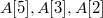 and
and  are right from it. The second row of Figure 15.18 shows the elements of
  in decreasing order of their ranks.
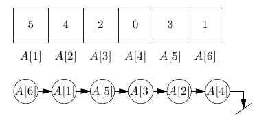
The list ranking problem can be solved in linear time using a sequential algorithm. At first we determine the head of the list which is the unique  having the property that does not exist an index
  with
with  . In our case the head of
  is
is  . The head of the list has the rank
  , its right neighbour has a rank
  and finally the rank of the last element is zero.
In this subsection we present a deterministic list ranking algorithm, which uses  EREW PRAM processors and in worst case
  time. The pseudocode of algorithm
 Det-Ranking is as follows.
The input of the algorithm is the number of the elements to be ranked  , the array
  containing the index of the right neighbour of the elements of
  , output is the array
  containing the computed ranks.
Det-Ranking(
)
1IN PARALLEL FOR
TO2
DOIF3
THEN4
ELSE5
FOR
TO6
DO
IN PARALLEL FOR
TO7
DOIF8
THEN9
10
RETURN

The basic idea behind the algorithm Det-Ranking is the pointer jumping. According to this algorithm at the beginning each element contains the index of its right neighbour, and accordingly its provisional rank equal to 1 (with exception of the last element of the list, whose rank equals to zero). This initial state is represented in the first row of Figure 15.19.
Then the algorithm modifies the element so, that each element points to the right neighbour of its right neighbour (if it exist, otherwise to the end of the list). This state is represented in the second row of Figure 15.19.
If we have  processors, then it can be done in
  time. After this each element (with exception of the last one) shows to the element whose distance was originally two. In the next step of the pointer jumping the elements will show to such other element whose distance was originally 4 (if there is no such element, then to the last one), as it is shown in the third row of Figure 15.19.
In the next step the pointer part of the elements points to the neighbour of distance 8 (or to the last element, if there is no element of distance 8), according to the last row of Figure 15.19.
In each step of the algorithm each element updates the information on the number of elements between itself and the element pointed by the pointer. Let  , resp.
  the rank, resp. neighbour field of the element
  . The initial value of
  is 1 for the majority of the elements, but is 0 for the rightmost element (
 in the first line of Figure 15.19). During the pointer jumping
  gets the new value (if
  ) gets the new value
  , if
, if  . E.g. in the second row of Figure 15.19)
  , since its previous rank is 1, and the rank of its right neighbour is also 1. After this
  will be modified to point to
  . E.g. in the second row of Figure 15.19
  , since the right neighbour of the right neighbour of
  is
is  .
.
Theorem 15.4 Algorithm Det-Ranking computes the ranks of an array consisting of  elements on
EREW PRAM processors in  time.
time.
Since the work of Det-Ranking is  , this algorithm is not work-optimal, but it is work-efficient.
The list ranking problem corresponds to a list prefix problem, where each element is 1, but the last element of the list is 0. One can easily modify Det-Ranking to get a prefix algorithm.
The input of the merging problem is two sorted sequences  and
and  and the output is one sorted sequence
  containing the elements of the input.
If the length of the input sequences is  , then the merging problem can be solved in
  time using a sequential processor. Since we have to investigate all elements and write them into the corresponding element of
  , the running time of any algorithm is
  . We get this lower bound even in the case when we count only the number of necessary comparisons.
Let  and
and  be the input sequences. For the shake of simplicity let
  be the power of two and let the elements be different.
To merge two sequences of length  it is enough to know the ranks of the keys, since then we can write the keys—using
  processors—into the corresponding memory locations with one parallel write operation. The running time of the following algorithm is a logarithmic, therefore it is called
 Logarithmic-Merge.
Theorem 15.5 Algorithm Logarithmic-Merge merges two sequences of length  on
on 
CREW PRAM processors in  time.
time.
Proof. Let the rank of element  be
be  in
in  (in
(in  ). If
). If  , then let
  . If we assign a single processor
  to the element
  , then it can determine, using binary search, the number
  of elements in
  , which are smaller than
  . If
. If  is known, then
  computes the rank
  in the union of
  and
and  , as
, as  . If
. If  belongs to
  , the method is the same.
Summarising the time requirements we get, that using one CREW PRAM processor per element, that is totally  processors the running time is
  .
.
This algorithm is not work-optimal, only work-efficient.
This following recursive algorithm Odd-Even-Merge follows the classical divide-and-conquer principle.
Let  and
and  be the two input sequences. We suppose that
  is a power of 2 and the elements of the arrays are different. The output of the algorithm is the sequence
  , containing the merged elements. This algorithm requires
  EREW PRAM processors.
Odd-Even-Merge(
)
1IF2
THENgetby merging
and
with one comparison 3
RETURN4
IF5
THEN
IN PARALLEL FOR
TO6
DOmerge recursivelyand 7
to get
8

IN PARALLEL FOR
TO9
DOmerge recursivelyand 10
to get
11

IN PARALLEL FOR
TO12
DO13
14
IF15
THEN16
17
18
RETURN
Example 15.5 Merge of twice eight numbers. Let  = 1, 5, 8, 11, 13, 16, 21, 26 and
  = 3, 9, 12, 18, 23, 27, 31, 65. Figure 15.20 shows the sort of 16 numbers.
At first elements of  with odd indices form the sequence
  and elements with even indices form the sequence
  , and in the same way we get the sequences
  and
and  . Then comes the recursive merge of the two odd sequences resulting
  and the recursive merge of the even sequences resulting
  .
.
After this Odd-Even-Merge shuffles  and
and  , resulting the sequence
  : the elements of
  with odd indices come from
  and the elements with even indices come from
  .
.
Finally we compare the elements of  with even index and the next element (that is
  with
with  ,
,  with
with  etc.) and if necessary (that is they are not in the good order) they are changed.
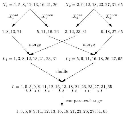
Theorem 15.6 (merging in  time) Algorithm
 Odd-Even-Merge merges two sequences of length  elements in
  time using
EREW PRAM processors.
Proof. Let denote the running time of the algorithm by  . Step 1 requires
  time, Step 2
  time. Therefore we get the recursive equation

having the solution  .
.
We prove the correctness of this algorithm using the zero-one principle.
A comparison-based sorting algorithm is oblivious, if the sequence of comparisons is fixed (elements of the comparison do not depend on the results of the earlier comparisons). This definition means, that the sequence of the pairs of elements to be compared  is given.
Theorem 15.7 (zero-one principle) If a simple comparison-based sorting algorithm correctly sorts an arbitrary 0-1 sequence of length n, then it sorts also correctly any sequence of length n consisting of arbitrary keys.
Proof. Let A be a comparison-based oblivious sorting algorithm and let  be such a sequence of elements, sorted incorrectly by A. Let suppose A sorts in increasing order the elements of
  . Then the incorrectly sorted sequence
  contains an element
  on the
  -th
-th  position in spite of the fact that
  contains at least
  keys smaller than
  .
.
Let  be the first (having the smallest index) such element of
  . Substitute in the input sequence the elements smaller than
  by 0's and the remaining elements by 1's. This modified sequence is a 0-1 sequence therefore A sorts it correctly. This observation implies that in the sorted 0-1 sequence at least
  0's precede the 1, written on the place of
  .
.
Now denote the elements of the input sequence smaller than  by red colour, and the remaining elements by blue colour (in the original and the transformed sequence too). We can show by induction, that the coloured sequences are identical at the start and remain identical after each comparison. According to colours we have three types of comparisons: blue-blue, red-red and blue-red. If the compared elements have the same colour, in both cases (after a change or not-change) the colours remain unchanged. If we compare elements of different colours, then in both sequences the red element occupy the position with smaller index. So finally we get a contradiction, proving the assertion of the theorem.
Example 15.6 A non comparison-based sorting algorithm. Let  be a bit sequence. We can sort this sequence simply counting the zeros, and if we count
  zeros, then write
  zeros, then
  ones. Of course, the general correctness of this algorithm is not guaranteed. Since this algorithm is not comparison-based, therefore this fact does not contradict to the zero-one principle.
But merge is sorting, and Odd-Even-Merge is an oblivious sorting algorithm.
Theorem 15.8 Algorithm Odd-Even-Merge sorts correctly sequences consisting of arbitrary numbers.
Proof. Let  and
and  sorted 0-1 sequences of length
  . Let
. Let  the number of zeros at the beginning of
  . Then the number of zeros in
  equals to
  , while the number of zeros in
  is
is  . Therefore the number of zeros in
  equals to
  and the number of zeros in
  equals to
  .
.
The difference of  and
and  is at most 2. This difference is exactly then 2, if
  and
and  are both odd numbers. Otherwise the difference is at most 1. Let suppose, that
  (the proof in the other cases is similar). In this cases
  contains two additional zeros. When the algorithm shuffles
  and
and  ,
,  begins with an even number of zeros, end an even number of ones, and between the zeros and ones is a short “dirty” part, 0, 1. After the comparison and change in the last step of the algorithm the whole sequence become sorted.
Algorithm Work-Optimal-Merge uses only  processors, but solves the merging in logarithmic time. This algorithm divides the original problem into
  parts so, that each part contains approximately
  elements.
Let  and
and  be the input sequences. Divide
  into
into  parts so, that each part contain at most
  elements. Let the parts be denoted by
  . Let the largest element in
  be
be  .
.
Assign a processor to each  element. These processors determine (by binary search) the correct place (according to the sorting) of
  in
in  . These places divide
  to
to  parts (some of these parts can be empty). Let denote these parts by
  . We call
  the subset corresponding to
  in
in  (see Figure 15.21).
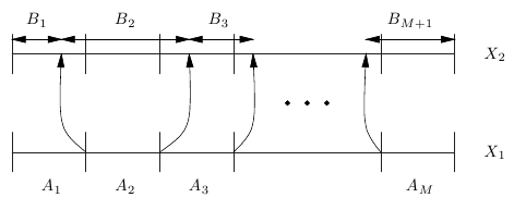
The algorithm gets the merged sequence merging at first  with
with  ,
,  with
with  and so on, and then joining these merged sequences.
Theorem 15.9 Algorithm Optimal-Merging merges two sorted sequences of length  in
in  time on
CREW PRAM processors.
Proof. We use the previous algorithm.
The length of the parts  is
is  , but the length of the parts
  can be much larger. Therefore we repeat the partition. Let
  an arbitrary pair. If
  , then
  and
and  can be merged using one processor in
  time. But if
  , then divide
  into
into  parts—then each part contains at most
  keys. Assign a processor to each part. This assigned processor finds the subset corresponding to this subsequence in
  :
:  time is sufficient to do this. So the merge of
  and
and  can be reduced to
  subproblems, where each subproblem is the merge of two sequences of
  length.
The number of the used processors is  , and this is at most
  , what is not larger then
  .
.
This theorem imply, that Optimal-Merging is work-optimal.
In the selection problem  elements and a positive integer
  are given and the
  -th smallest element is to be selected. Since selection requires the investigation of all elements, and our operations can handle at most two elements, so
  .
.
Since it is known sequential algorithm A requiring only  time, so A is asymptotically optimal.
The search problem is similar: in that problem the algorithm has to decide, whether a given element appears in the given sequence, and if yes, then where. Here negative answer is also possible and the features of any element decide, whether it corresponds the requirements or not.
We investigate three special cases and work-efficient algorithms to solve them.
 processors.
Let  , that is we wish to select the largest key. Algorithm
 Quadratic-Select solves this task in  time using
  CRCW processors.
The input ( different keys) is the sequence
  , and the selected largest element is returned as
  .
.
Quadratic-Select(
)
1IF2
THEN3
RETURN4

IN PARALLEL FOR
TO,

TO
DOIF5
THENFALSE6ELSETRUE7
IN PARALLEL FOR
TO8
DOTRUE9
IN PARALLEL FOR
TO,

TO10
IFFALSE11THENFALSE12
IN PARALLEL FOR
TO13
DOIFTRUE14THEN15
RETURN


In the first round (lines 4–6) the keys are compared in parallel manner, using all the  processors.
  so, that processor
  computes the logical value
  . We suppose that the keys are different. If the elements are not different, then we can use instead of
  the pair
  (this solution requires an additional number of length
  bits. Since there is a unique key for which all comparison result
 FALSE, this unique key can be found with a logical OR operation is lines 7–11.
Theorem 15.11 (selection in  time) Algorithm
 Quadratic-Select determines the largest key of  different keys in
  time using
CRCW common PRAM processors.
Proof. First and third rounds require unit time, the second round requires  time, so the total running time is
  .
.
The speedup of this algorithm is  . The work of the algorithm is
  . So the efficiency is
  . It follows that this algorithm is not work-optimal, even it is not work-effective.
 processors.
Now we show that the maximal element among  keys can be found, using even only
  common CRCW PRAM processors and
  time. The used technique is the divide-and-conquer. For the simplicity let
  be a square number.
The input and the output are the same as at the previous algorithm.
Quick-Selection(
)
1IF2
THEN3
RETURN4
IF5
THENdivide the input into groupsand divide the processors into groups
6

IN PARALLEL FOR
TO7
DOrecursively determines the maximal elementof the group
8
Quadratic-Select()9RETURN

The algorithm divides the input into  groups
  so, that each group contains
  elements
  , and divides the processors into
  groups
  so, that group
  contains
  processors
  . Then the group of processors
  computes recursively the maximum
  of group
  . Finally the previous algorithm
 Quadratic-Select gets as input the sequence  and finds the maximum y of the input sequence
  .
.
Theorem 15.12 (selection in  time) Algorithm
 Quick-Select determines the largest of  different elements in
  time using
  common
 CRCW PRAM processors.
Let the running time of the algorithm denoted by  . Step 1 requires
  time, step 2 requires
  time. Therefore
  satisfies the recursive equation

having the solution  .
.
The total work of algorithm Quick-Select is  , so its efficiency is
  , therefore
 Quick-Select is not work-optimal, it is only work-effective.
If the problem is to find the maximum of  keys when the keys consist of one bit, then the problem can be solved using a logical
 OR operation, and so requires only constant time using  processors. Now we try to extend this observation. Let
  be a given positive integer constant, and we suppose the keys are integer numbers, belonging to the interval
  . Then the keys can be represented using at most
  bits. For the simplicity we suppose that all the keys are given as binary numbers of length
  bits.
bits.
The following algorithm Integer-Selection requires only constant time and  CRCW PRAM processors to find the maximum.
The basic idea is to partition the  bits of the numbers into parts of length
  . The
. The  -th part contains the bits
  , the number of the parts is
  . Figure 15.22 shows the partition.
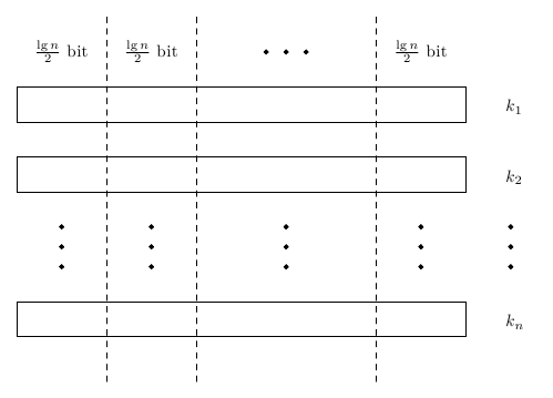
The input of Integer-Selection is the number of processors  and the sequence
  containing different integer numbers, and output is the maximal number
  .
.
Integer-Selection(
)
1FOR
TO2
DOcompute the maximumof the remaining numbers on the base of their
-th part 3 delete the numbers whose
-th part is smaller than
4
one of the remaining numbers 5
RETURN
The algorithm starts with searching the maximum on the base of the first part of the numbers. Then it delete the numbers, whose first part is smaller, than the maximum. Then this is repeated for the second, ..., last part of the numbers. Any of the non deleted numbers is maximal.
Theorem 15.13 (selection from integer numbers) If the numbers are integers drawn from the interval  , then algorithm
 Integer-Selection determines the largest number among  numbers for any positive
  in
in  time using
CRCW PRAM processors.
Proof. Let suppose that we start with the selection of numbers, whose  most significant bits are maximal. Let this maximum in the first part denoted by
  . It is sure that the numbers whose first part is smaller than
  are not maximal, therefore can be deleted. If we execute this basis operation for all parts (that is
  times), then exactly those numbers will be deleted, what are not maximal, and all maximal element remain.
If a key contains at most  bits, then its value is at most
  . So algorithm
 Integer-Select in its first step determines the maximum of integer numbers taken from the interval  . The algorithm assigns a processor to each number and uses
  common memory locations
  , containing initially
  . In one step processor
  writes
  into
into  . Later the maximum of all numbers can be determined from
  memory cells using
  processors by Theorem 15.11 in constant time.
Let the sequence  contain different numbers and the problem is to select the
  th smallest element of
  . Let we have
  CREW processors.
General-Selection(
)
1 divide theprocessors into
groups
so, that group
contains the processors
and divide the
elements into
groups
so, that group
contains the elements
2

IN PARALLEL FOR
TO3
DOdetermine(how many elements of
are smaller, than
) 4

IN PARALLEL FOR
TO5
DOusingOptimal-Prefixdetermine(how many elements of
are smaller, than
) 6

IN PARALLEL FOR
TO7
DOIF8
THEN RETURN
Theorem 15.14 (general selection) The algorithm General-Selection determines the  -th smallest of
  different numbers in
  time using
  processors.
Proof. In lines 2–3  works as a sequential processor, therefore these lines require
  time. Lines 4–5 require
  time according to Theorem 15.3. Lines 6–8 can be executed in constant time, so the total running time is
  .
.
The work of General-Selection is  , therefore this algorithm is not work-effective.
Given a sequence  the sorting problem is to rearrange the elements of
  e.g. in increasing order.
It is well-known that any A sequential comparison-based sorting algorithm needs  comparisons, and there are comparison-based sorting algorithms with
  running time.
There are also algorithms, using special operations or sorting numbers with special features, which solve the sorting problem in linear time. If we have to investigate all elements of  and permitted operations can handle at most 2 elements, then we get
  . So it is true, that among the comparison-based and also among the non-comparison-based sorting algorithms are asymptotically optimal sequential algorithms. In this subsection we consider three different sorting algorithm.
 processors.
Using the ideas of algorithms Quadratic-Selection and Optimal-Prefix we can sort  elements using
  processors in
  time.
time.
Quadratic-Sort(
)
1IF2
THEN3
RETURN4

IN PARALLEL FOR
TO,

TO
DOIF5
THEN6
ELSE7 divide the processors into
groups
so, that group
contains processors
8

IN PARALLEL FOR
TO9
DOcompute10

IN PARALLEL FOR
TO11
DO12
RETURN
In lines 4–7 the algorithm compares all pairs of the elements (as Quadratic-Selection), then in lines 7–9 (in a similar way as Optimal-Prefix works) it counts, how many elements of  is smaller, than the investigated
  , and finally in lines 10–12 one processor of each group writes the final result into the corresponding memory cell.
Theorem 15.15 (sorting in  time) Algorithm
 Quadratic-Sort sorts  elements using
CRCW PRAM processors in  time.
time.
Proof. Lines 8–9 require  time, and the remaining lines require only constant time.
Since the work of Quadratic-Sort is  , this algorithm is not work-effective.
 running time.
The next algorithm uses the Odd-Even-Merge algorithm and the classical divide-and-conquer principle. The input is the sequence  , containing the numbers to be sorted, and the output is the sequence
  , containing the sorted numbers.
Odd-Even-Sort(
)
1IF2
THEN3
IF4
THENletand
. 5

IN PARALLEL FOR
TO6
DOsort recursivelyto get
7

IN PARALLEL FOR
TO8
DOsort recursivelyto get
9

IN PARALLEL FOR
TO10
DOmergeand
using
Odd-Even-Merge()11RETURN

The running time of this EREW PRAM algorithm is  .
.
Theorem 15.16 (sorting in  time) Algorithm
 Odd-Even-Sort sorts  elements in
  time using
EREW PRAM processors.
Proof. Let  be the running time of the algorithm. Lines 3–4 require
  time, Lines 5–8 require
  time, and lines 9–10 require
  time, line 11 require
  time. Therefore
  satisfies the recurrence

having the solution  .
.
Example 15.7 Sorting on 16 processors. Sort using 16 processors the following numbers: 62, 19, 8, 5, 1, 13, 11, 16, 23, 31, 9, 3, 18, 12, 27, 34. At first we get the odd and even parts, then the first 8 processors gets the sequence  , while the other 8 processors get
  . The output of the first 8 processors is
  , while the output of the second 8 processors is
  . The merged final result is
  .
.
The work of the algorithm is  , its efficiency is
  , and its speedup is
  . The algorithm is not work-optimal, but it is work-effective.
 running time.
If we have more processors, then the running time can be decreased. The following recursive algorithm due to Preparata uses  CREW PRAM processors and
  time. Input is the sequence
  , and the output is the sequence
  containing the sorted elements.
Preparata(
)
1IF2
THENsortusing
processors and
Odd-Even-Sort3RETURN4 divide the
elements into
parts
so, that each part contains
elements, and divide the processors into
groups
so, that each group contains
processors 5

IN PARALLEL FOR
TO6
DOsort the partrecursively to get a sorted sequence
7 divide the processors into
groups
containing
processors 8

IN PARALLEL FOR
TO
TO9
DOmergeand
10 divide the processors into
groups
so, that each group contains
processors 11

IN PARALLEL FOR
TO12
DOdetermine the ranks of theelement in
using the local ranks received in line 9 and using the algorithm
Optimal-Prefix13the elements of
having a rank
14
RETURN
This algorithm uses the divide-and-conquer principle. It divides the input into  parts, then merges each pair of parts. This merge results local ranks of the elements. The global rank of the elements can be computed summing up these local ranks.
Theorem 15.17 (sorting in  time) Algorithm
 Preparata sorts  elements in
  time using
CREW PRAM processors.
Proof. Let the running time be  . Lines 4–6 require
  time, lines 7–12 together
  . Therefore
  satisfies the equation

having the solution  .
.
The work of Preparata is the same, as the work of Odd-Even-Sort, but the speedup is better:  . The efficiency of both algorithms is
  .
.
Exercises
15.6-1 The memory cell  of the global memory contains some data. Design an algorithm, which copies this data to the memory cells
  in
in  time, using
  EREW PRAM processors.
15.6-2 Design an algorithm which solves the previous Exercise 15.6-1 using only  EREW PRAM processors saving the
  running time.
15.6-3 Design an algorithm having  running time and determining the maximum of
  numbers using
  common CRCW PRAM processors.
15.6-4 Let  be a sequence containing
  keys. Design an algorithm to determine the rank of any
  key using
  CREW PRAM processors and
  time.
time.
15.6-5 Design an algorithm having  running time, which decides using
  common CRCW PRAM processors, whether element 5 is contained by a given array
  , and if is contained, then gives the largest index
  , for which
  holds.
15.6-6 Design algorithm to merge two sorted sequence of length  in
in  time, using
  CREW PRAM processors.
15.6-7 Determine the running time, speedup, work, and efficiency of all algorithms, discussed in this section.
To illustrate another model of computation we present two algorithms solving the prefix problem on meshes.
Let suppose that processor  of the chain
  stores element
  in its local memory, and after the parallel computations the prefix
  will be stored in the local memory of
  . At first we introduce a naive algorithm. Its input is the sequence of elements
  , and its output is the sequence
  , containing the prefixes.
Chain-Prefix(
)
1sends
to
2

IN PARALLEL FOR
TO3
FOR
TO4
DOgetsfrom
, then computes and stores
stores
, and sends
to
5
gets
from
, then computes and stores
Saying the truth, this is not a real parallel algorithm.
Theorem 15.18 Algorithm Chain-Prefix determines the prefixes of p elements using a chain  in
in  time.
time.
Proof. The cycle in lines 2–5 requires  time, line 1 and line 6 requires
  time.
time.
Since the prefixes can be determined in  time using a sequential processor, and
  , so
, so CHAIN-Prefix is not work-effective.
An algorithm, similar to Chain-Prefix, can be developed for a square too.
Let us consider a square of size  . We need an indexing of the processors. There are many different indexing schemes, but for the next algorithm
 Square-Prefix sufficient is the one of the simplest solutions, the row-major indexing scheme, where processor  gets the index
  .
.
The input and the output are the same, as in the case of Chain-Prefix.
The processors  form the processor row
  and the processors
  form the processor column
  . The input stored by the processors of row
  is denoted by
  , and the similar output is denoted by
  .
.
The algorithm works in 3 rounds. In the first round (lines 1–8) processor rows  compute the row-local prefixes (working as processors of
 Chain-Prefix). In the second round (lines 9–17) the column  computes the prefixes using the results of the first round, and the processors of this column
  send the computed prefix to the neighbour
  . Finally in the third round the rows
  determine the final prefixes.
Square-Prefix(
)
1
IN PARALLEL FOR
TO2
DOsendsto
3

IN PARALLEL FOR
TO4
FOR
TO5
DOgetsfrom
, then computes and 6 stores
, and sends
to
7

IN PARALLEL FOR
TO8
DOgetsfrom
, then computes and stores
9
sends
to
10

IN PARALLEL FOR
TO11
FOR
TO12
DOgetsfrom
, then computes and stores stores
, and sends
to
13
gets
from
, then computes and stores
14

IN PARALLEL FOR
TO15
DOsendto
16

IN PARALLEL FOR
TO17
DOsendsto
18

IN PARALLEL FOR
DOWNTO19
FOR
TO20
DOgetsfrom
, then computes and 21 stores
, and sends
to
22

IN PARALLEL FOR
TO23
DOgetsfrom
, then computes and stores
Theorem 15.19 Algorithm Square-Prefix solves the prefix problem using a square of size  , major row indexing in
  time.
time.
Proof. In the first round lines 1–2 contain 1 parallel operation, lines 3–6 require  operations, and line 8 again 1 operation, that is all together
  operations. In a similar way in the third round lines 18–23 require
  time units, and in round 2 lines 9–17 require
  time units. The sum of the necessary time units is
  .
.
Example 15.8 Prefix computation on square of size  Figure 15.23(a) shows 16 input elements. In the first round
 Square-Prefix computes the row-local prefixes, part (b) of the figure show the results. Then in the second round only the processors of the fourth column work, and determine the column-local prefixes – results are in part (c) of the figure. Finally in the third round algorithm determines the final results shown in part (d) of the figure.
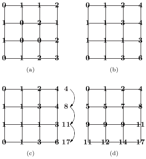
CHAPTER NOTES |
Basic sources of this chapter are for architectures and models the book of Leopold [221], and the book of Sima, Fountaine and Kacsuk [304], for parallel programming the book due to Kumar et al. [141] and [221], for parallel algorithms the books of Berman and Paul, [41] Cormen, Leiserson and Rivest [72], the book written by Horowitz, Sahni and Rajasekaran [167] and the book [176], and the recent book due to Casanova, Legrand and Robert [58].
The website [324] contains the Top 500 list, a regularly updated survey of the most powerful computers worldwide [324]. It contains 42% clusters.
Described classifications of computers are proposed by Flynn [113], and Leopold [221]. The Figures 15.1, 15.2, 15.3, 15.4, 15.5, 15.7 are taken from the book of Leopold [221], the program 15.6 from the book written by Gropp et al. [145].
The clusters are characterised using the book of Pfister [273], grids are presented on the base of the book and manuscript of Foster and Kellerman [117], [118].
With the problems of shared memory deal the book written by Hwang and Xu [172], the book due to Kleiman, Shah, and Smaalders [199], and the textbook of Tanenbaum and van Steen [315].
Details on concepts as tasks, processes and threads can be found in many textbook, e.g. in [303], [314]. Decomposition of the tasks into smaller parts is analysed by Tanenbaum and van Steen [315].
The laws concerning the speedup were described by Amdahl [15], Gustafson-Barsis [150] and Brent [47]. Kandemir, Ramanujam and Choudray review the different methods of the improvement of locality [188]. Wolfe [346] analyses in details the connection between the transformation of the data and the program code. In connection with code optimisation the book published by Kennedy and Allen [197] is a useful source.
The MPI programming model is presented according to Gropp, Snir, Nitzberg, and Lusk [145], while the base of the description of the OpenMP model is the paper due to Chandra, Dragum, Kohr, Dror, McDonald and Menon [60], further a review found on the internet [258].
Lewis and Berg [222] discuss pthreads, while Oaks and Wong [257] the Java threads in details. Description of High Performance Fortran can be found in the book Koelbel et al. [204]. Among others Wolfe [346] studied the parallelising compilers.
The concept of PRAM is due to Fortune and Wyllie and is known since 1978 [116]. BSP was proposed in 1990 by Valiant [334]. LogP has been suggested as an alternative of BSP by Culler et al. in 1993 [78]. QSM was introduced in 1999 by Gibbons, Matias and Ramachandran [132].
The majority of the pseudocode conventions used in Section 15.6 and the description of crossover points and comparison of different methods of matrix multiplication can be found in [72].
The Readers interested in further programming models, as skeletons, parallel functional programming, languages of coordination and parallel mobile agents, can find a detailed description in [221]. Further problems and parallel algorithms are analysed in the books of Leighton [218], [219] and in the chapter Memory Management of this book [28] and in the book of Horowitz, Sahni and Rajasekaran [167]. A model of scheduling of parallel processes is discussed in [130], [174], [345].
Cost-optimal parallel merge is analysed by Wu and Olariu in [349]. New ideas (as the application of multiple comparisons to get a constant time sorting algoritm) of parallel sorting can be found in the paper of Gararch, Golub and Kruskal [126].
Table of Contents
Systolic arrays probably constitute a perfect kind of special purpose computer. In their simplest appearance, they may provide only one operation, that is repeated over and over again. Yet, systolic arrays show an abundance of practice-oriented applications, mainly in fields dominated by iterative procedures: numerical mathematics, combinatorial optimisation, linear algebra, algorithmic graph theory, image and signal processing, speech and text processing, et cetera.
For a systolic array can be tailored to the structure of its one and only algorithm thus accurately! So that time and place of each executed operation are fixed once and for all. And communicating cells are permanently and directly connected, no switching required. The algorithm has in fact become hardwired. Systolic algorithms in this respect are considered to be hardware algorithms. Please note that the term systolic algorithms usually does not refer to a set of concrete algorithms for solving a single specific computational problem, as for instance sorting. And this is quite in contrast to terms like sorting algorithms. Rather, systolic algorithms constitute a special style of specification, programming, and computation. So algorithms from many different areas of application can be systolic in style. But probably not all well-known algorithms from such an area might be suited to systolic computation.
Hence, this chapter does not intend to present all systolic algorithms, nor will it introduce even the most important systolic algorithms from any field of application. Instead, with a few simple but typical examples, we try to lay the foundations for the Readers' general understanding of systolic algorithms. The rest of this chapter is organised as follows: Section 16.1 shows some basic concepts of systolic systems by means of an introductory example. Section 16.2 explains how systolic arrays formally emerge from space-time transformations. Section 16.3 deals with input/output schemes. Section 16.4 is devoted to all aspects of control in systolic arrays. In Section 16.5 we study the class of linear systolic arrays, raising further questions.
The designation systolic follows from the operational principle of the systolic architecture. The systolic style is characterised by an intensive application of both pipelining and parallelism, controlled by a global and completely synchronous clock. Data streams pulsate rhythmically through the communication network, like streams of blood are driven from the heart through the veins of the body. Here, pipelining is not constrained to a single space axis but concerns all data streams possibly moving in different directions and intersecting in the cells of the systolic array.
A systolic system typically consists of a host computer, and the actual systolic array. Conceptionally, the host computer is of minor importance, just controlling the operation of the systolic array and supplying the data. The systolic array can be understood as a specialised network of cells rapidly performing data-intensive computations, supported by massive parallelism. A systolic algorithm is the program collaboratively executed by the cells of a systolic array.
Systolic arrays may appear very differently, but usually share a couple of key features: discrete time scheme, synchronous operation, regular (frequently two-dimensional) geometric layout, communication limited to directly neighbouring cells, and spartan control mechanisms.
In this section, we explain fundamental phenomena in context of systolic arrays, driven by a running example. A computational problem usually allows several solutions, each implemented by a specific systolic array. Among these, the most attractive designs (in whatever respect) may be very complex. Note, however, that in this educational text we are less interested in advanced solutions, but strive to present important concepts compactly and intuitively.
Figure 16.1 shows a rectangular systolic array consisting of 15 cells for multiplying a  matrix
  by an
by an  matrix
  . The parameter
  is not reflected in the structure of this particular systolic array, but in the input scheme and the running time of the algorithm.
The input scheme depicted is based on the special choice of parameter  . Therefore, Figure 16.1 gives a solution to the following problem instance:

where
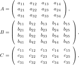
and
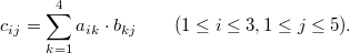
The cells of the systolic array can exchange data through links, drawn as arrows between the cells in Figure 16.1(a). Boundary cells of the systolic array can also communicate with the outside world. All cells of the systolic array share a common connection pattern for communicating with their environment. The completely regular structure of the systolic array (placement and connection pattern of the cells) induces regular data flows along all connecting directions.
Figure 16.1(b) shows the internal structure of a cell. We find a multiplier, an adder, three registers, and four ports, plus some wiring between these units. Each port represents an interface to some external link that is attached to the cell. All our cells are of the same structure.
Each of the registers A, B, C can store a single data item. The designations of the registers are suggestive here, but arbitrary in principle. Registers A and B get their values from input ports, shown in Figure 16.1(b) as small circles on the left resp. upper border of the cell.
The current values of registers A and B are used as operands of the multiplier and, at the same time, are passed through output ports of the cell, see the circles on the right resp. lower border. The result of the multiplication is supplied to the adder, with the second operand originating from register C. The result of the addition eventually overwrites the past value of register C.
Figure 16.1. Rectangular systolic array for matrix product. (a) Array structure and input scheme. (b) Cell structure.
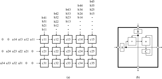
The 15 cells of the systolic array are organised as a rectangular pattern of three rows by five columns, exactly as with matrix  . Also, these dimensions directly correspond to the number of rows of matrix
  and the number of columns of matrix
  . The size of the systolic array, therefore, corresponds to the size of some data structures for the problem to solve. If we had to multiply an
  matrix
  by an
by an  matrix
  in the general case, then we would need a systolic array with
  rows and
  columns.
The quantities  are parameters of the problem to solve, because the number of operations to perform depends on each of them; they are thus problem parameters. The size of the systolic array, in contrast, depends on the quantities
  and
and  , only. For this reason,
  and
and  become also array parameters, for this particular systolic array, whereas
  is not an array parameter.
Remark. For matrix product, we will see another systolic array in Section 16.2, with dimensions dependent on all three problem parameters  .
.
An  systolic array as shown in Figure 16.1 would also permit to multiply an
  matrix
  by an
by an  matrix
  , where
  and
and  . This is important if we intend to use the same systolic array for the multiplication of matrices of varying dimensions. Then we would operate on a properly dimensioned rectangular subarray, only, consisting of
  rows and
  columns, and located, for instance, in the upper left corner of the complete array. The remaining cells would also work, but without any contribution to the solution of the whole problem; they should do no harm, of course.
Now let's assume that we want to assign unique space coordinates to each cell of a systolic array, for characterising the geometric position of the cell relative to the whole array. In a rectangular systolic array, we simply can use the respective row and column numbers, for instance. The cell marked with  in Figure 16.1 thus would get the coordinates (1,1), the cell marked with
  would get the coordinates (1,2), cell
  would get (2,1), and so on. For the remainder of this section, we take space coordinates constructed in such a way for granted.
In principle it does not matter where the coordinate origin lies, where the axes are pointing to, which direction in space corresponds to the first coordinate, and which to the second. In the system presented above, the order of the coordinates has been chosen corresponding to the designation of the matrix components. Thus, the first coordinate stands for the rows numbered top to bottom from position 1, the second component stands for the columns numbered left to right, also from position 1.
Of course, we could have made a completely different choice for the coordinate system. But the presented system perfectly matches our particular systolic array: the indices of a matrix element  computed in a cell agree with the coordinates of this cell. The entered rows of the matrix
  carry the same number as the first coordinate of the cells they pass; correspondingly for the second coordinate, concerning the columns of the matrix $B$. All links (and thus all passing data flows) are in parallel to some axis, and towards ascending coordinates.
It is not always so clear how expressive space coordinates can be determined; we refer to the systolic array from Figure 16.3(a) as an example. But whatsoever the coordinate system is chosen: it is important that the regular structure of the systolic array is obviously reflected in the coordinates of the cells. Therefore, almost always integral coordinates are used. Moreover, the coordinates of cells with minimum Euclidean distance should differ in one component, only, and then with distance 1.
Each active cell  from Figure 16.1 computes exactly the element
  of the result matrix
  . Therefore, the cell must evaluate the dot product

This is done iteratively: in each step, a product  is calculated and added to the current partial sum for
  . Obviously, the partial sum has to be cleared—or set to another initial value, if required—before starting the accumulation. Inspired by the classical notation of imperative programming languages, the general proceeding could be specified in pseudocode as follows:
Matrix-Product(
)
1FOR
TO2
DOFOR
TO3
DO4
FOR
TO5
DO6
RETURN
If  , we have to perform
  multiplications, additions, and assignments, each. Hence the running time of this algorithm is of order
  for any sequential processor.
The sum operator  is one of the so-called generic operators, that combine an arbitrary number of operands. In the systolic array from Figure 16.1, all additions contributing to a particular sum are performed in the same cell. However, there are plenty of examples where the individual operations of a generic operator are spread over several cells—see, for instance, the systolic array from Figure 16.3.
Remark. Further examples of generic operators are: product, minimum, maximum, as well as the Boolean operators AND, OR, and EXCLUSIVE OR.
Thus, generic operators usually have to be serialised before the calculations to perform can be assigned to the cells of the systolic array. Since the distribution of the individual operations to the cells is not unique, generic operators generally must be dealt with in another way than simple operators with fixed arity, as for instance the dyadic addition.
Instead of using an imperative style as in algorithm Matrix-product, we better describe systolic programs by an assignment-free notation which is based on an equational calculus. Thus we avoid side effects and are able to directly express parallelism. For instance, we may be bothered about the reuse of the program variable  from algorithm
 Matrix-product. So, we replace  with a sequence of instances
  , that stand for the successive states of
  . This approach yields a so-called recurrence equation We are now able to state the general matrix product from algorithm
 Matrix-product by the following assignment-free expressions:
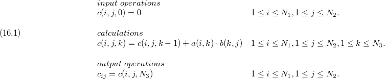
System (16.1) explicitly describes the fine structure of the executed systolic algorithm. The first equation specifies all input data, the third equation all output data. The systolic array implements these equations by input/output operations. Only the second equation corresponds to real calculations.
Each equation of the system is accompanied, on the right side, by a quantification. The quantification states the set of values the iteration variables  and
and  (and, for the second equation, also
  ) should take. Such a set is called a domain. The iteration variables
  of the second equation can be combined in an iteration vector
  . For the input/output equations, the iteration vector would consist of the components
  and
and  , only. To get a closed representation, we augment this vector by a third component
  , that takes a fixed value. Inputs then are characterised by
  , outputs by
  . Overall we get the following system:
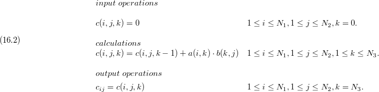
Note that although the domains for the input/output equations now are formally also of dimension 3, as a matter of fact they are only two-dimensional in the classical geometric sense.
From equations as in system (16.2), we directly can infer the atomic entities to perform in the cells of the systolic array. We find these operations by instantiating each equation of the system with all points of the respective domain. If an equation contains several suboperations corresponding to one point of the domain, these are seen as a compound operation, and are always processed together by the same cell in one working cycle.
In the second equation of system (16.2), for instance, we find the multiplication  and the successive addition
  . The corresponding elementary operations—multiplication and addition—are indeed executed together as a multiply-add compound operation by the cell of the systolic array shown in Figure 16.1(b).
Now we can assign a designation to each elementary operation, also called coordinates. A straight-forward method to define suitable coordinates is provided by the iteration vectors  used in the quantifications.
Applying this concept to system (16.1), we can for instance assign the tuple of coordinates  to the calculation
  . The same tuple
  is assigned to the input operation
  , but with setting
  . By the way: all domains are disjoint in this example.
If we always use the iteration vectors as designations for the calculations and the input/output operations, there is no further need to distinguish between coordinates and iteration vectors. Note, however, that this decision also mandates that all operations belonging to a certain point of the domain together constitute a compound operation—even when they appear in different equations and possibly are not related. For simplicity, we always use the iteration vectors as coordinates in the sequel.
The various elementary operations always happen in discrete timesteps in the systolic cells. All these timesteps driving a systolic array are of equal duration. Moreover, all cells of a systolic array work completely synchronous, i.e., they all start and finish their respective communication and calculation steps at the same time. Successive timesteps controlling a cell seamlessly follow each other.
Remark. But haven't we learned from Albert Einstein that strict simultaneity is physically impossible? Indeed, all we need here are cells that operate almost simultaneously. Technically this is guaranteed by providing to all systolic cells a common clock signal that switches all registers of the array. Within the bounds of the usually achievable accuracy, the communication between the cells happens sufficiently synchronised, and thus no loss of data occurs concerning send and receive operations. Therefore, it should be justified to assume a conceptional simultaneity for theoretical reasoning.
Now we can slice the physical time into units of a timestep, and number the timesteps consecutively. The origin on the time axis can be arbitrarily chosen, since time is running synchronously for all cells. A reasonable decision would be to take  as the time of the first input in any cell. Under this regime, the elementary compound operation of system (16.2) designated by
  would be executed at time
  . On the other hand, it would be evenly justified to assign the time
  to the coordinates
  ; because this change would only induce a global time shift by three time units.
So let us assume for the following that the execution of an instance  starts at time
  . The first calculation in our example then happens at time
  , the last at time
  . The running time thus amounts to
  timesteps.
Normally, the data needed for calculation by the systolic array initially are not yet located inside the cells of the array. Rather, they must be infused into the array from the outside world. The outside world in this case is a host computer, usually a scalar control processor accessing a central data storage. The control processor, at the right time, fetches the necessary data from the storage, passes them to the systolic array in a suitable way, and eventually writes back the calculated results into the storage.
Each cell  must access the operands
  and
and  during the timestep concerning index value
  . But only the cells of the leftmost column of the systolic array from Figure 16.1 get the items of the matrix
  directly as input data from the outside world. All other cells must be provided with the required values
  from a neighbouring cell. This is done via the horizontal links between neighbouring cells, see Figure 16.1(a). The item
  successively passes the cells
  . Correspondingly, the value
  enters the array at cell
  , and then flows through the vertical links, reaching the cells
  up to cell
  . An arrowhead in the figure shows in which direction the link is oriented.
Frequently, it is considered problematic to transmit a value over large distances within a single timestep, in a distributed or parallel architecture. Now suppose that, in our example, cell  got the value
  during timestep
  from cell
  , or from the outside world. For the reasons described above,
  is not passed from cell
  to cell
  in the same timestep
  , but one timestep later, i.e., at time
  . This also holds for the values
  . The delay is visualised in the detail drawing of the cell from Figure 16.1(b): input data flowing through a cell always pass one register, and each passed register induces a delay of exactly one timestep.
Remark. For systolic architectures, it is mandatory that any path between two cells contains at least one register—even when forwarding data to a neighbouring cell, only. All registers in the cells are synchronously switched by the global clock signal of the systolic array. This results in the characteristic rhythmical traffic on all links of the systolic array. Because of the analogy with pulsating veins, the medical term systole has been reused for the name of the concept.
To elucidate the delayed forwarding of values, we augment system (16.1) with further equations. Repeatedly used values like  are represented by separate instances, one for each access. The result of this proceeding—that is very characteristic for the design of systolic algorithms—is shown as system (16.3).
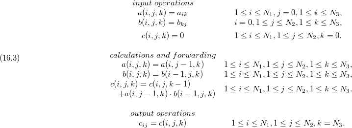
Each of the partial sums  in the progressive evaluation of
  is calculated in a certain timestep, and then used only once, namely in the next timestep. Therefore, cell
  must provide a register (named C in Figure 16.1(b)) where the value of
  can be stored for one timestep. Once the old value is no longer needed, the register holding
  can be overwritten with the new value
  . When eventually the dot product is completed, the register contains the value
  , that is the final result
  . Before performing any computation, the register has to be cleared, i.e., preloaded with a zero value—or any other desired value.
In contrast, there is no need to store the values  and
and  permanently in cell
  . As we can learn from Figure 16.1(a), each row of the matrix
  is delayed by one timestep with respect to the preceding row. And so are the columns of the matrix
  . Thus the values
  and
and  arrive at cell
  exactly when the calculation of
  is due. They are put to the registers A resp. B, then immediately fetched from there for the multiplication, and in the same cycle forwarded to the neighbouring cells. The values
  and
and  are of no further use for cell
  after they have been multiplied, and need not be stored there any longer. So A and B are overwritten with new values during the next timestep.
It should be obvious from this exposition that we urgently need to make economic use of the memory contained in a cell. Any calculation and any communication must be coordinated in space and time in such a way that storing of values is limited to the shortest-possible time interval. This goal can be achieved by immediately using and forwarding the received values. Besides the overall structure of the systolic array, choosing an appropriate input/output scheme and placing the corresponding number of delays in the cells essentially facilitates the desired coordination. Figure 16.1(b) in this respect shows the smallest possible delay by one timestep.
Geometrically, the input scheme of the example resulted from skewing the matrices  and
and  . Thereby some places in the input streams for matrix
  became vacant and had to be filled with zero values; otherwise, the calculation of the
  would have been garbled. The input streams in length depend on the problem parameter
  .
.
As can been seen in Figure 16.1, the items of matrix  are calculated stationary, i.e., all additions contributing to an item
  happen in the same cell. Stationary variables don't move at all during the calculation in the systolic array. Stationary results eventually must be forwarded to a border of the array in a supplementary action for getting delivered to the outside world. Moreover, it is necessary to initialise the register for item
  . Performing these extra tasks requires a high expenditure of runtime and hardware. We will further study this problem in Section 16.4.
The characteristic operating style with globally synchronised discrete timesteps of equal duration and the strict separation in time of the cells by registers suggest systolic arrays to be special cases of pipelined systems. Here, the registers of the cells correspond to the well-known pipeline registers. However, classical pipelines come as linear structures, only, whereas systolic arrays frequently extend into more spatial dimensions—as visible in our example. A multi-dimensional systolic array can be regarded as a set of interconnected linear pipelines, with some justification. Hence it should be apparent that basic properties of one-dimensional pipelining also apply to multi-dimensional systolic arrays.
A typical effect of pipelining is the reduced utilisation at startup and during shut-down of the operation. Initially, the pipe is empty, no pipeline stage active. Then, the first stage receives data and starts working; all other stages are still idle. During the next timestep, the first stage passes data to the second stage and itself receives new data; only these two stages do some work. More and more stages become active until all stages process data in every timestep; the pipeline is now fully utilised for the first time. After a series of timesteps at maximum load, with duration dependent on the length of the data stream, the input sequence ceases; the first stage of the pipeline therefore runs out of work. In the next timestep, the second stage stops working, too. And so on, until eventually all stages have been fallen asleep again. Phases of reduced activity diminish the average performance of the whole pipeline, and the relative contribution of this drop in productivity is all the worse, the more stages the pipeline has in relation to the length of the data stream.
We now study this phenomenon to some depth by analysing the two-dimensional systolic array from Figure 16.1. As expected, we find a lot of idling cells when starting or finishing the calculation. In the first timestep, only cell  performs some useful work; all other cells in fact do calculations that work like null operations—and that's what they are supposed to do in this phase. In the second timestep, cells
  and
and  come to real work, see Figure 16.2(a). Data is flooding the array until eventually all cells are doing work. After the last true data item has left cell
  , the latter is no longer contributing to the calculation but merely reproduces the finished value of
  . Step by step, more and more cells drop off. Finally, only cell
  makes a last necessary computation step; Figure 16.2(b) shows this concluding timestep.
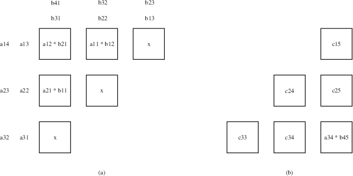
Exercises
16.1-1 What must be changed in the input scheme from Figure 16.1(a) to multiply a  matrix by a
  matrix on the same systolic array? Could the calculations be organised such that the result matrix would emerge in the lower right corner of the systolic array?
16.1-2 Why is it necessary to clear spare slots in the input streams for matrix  , as shown in Figure 16.1? Why haven't we done the same for matrix
  also?
also?
16.1-3 If the systolic array from Figure 16.1 should be interpreted as a pipeline: how many stages would you suggest to adequately describe the behaviour?
Although the approach taken in the preceding section should be sufficient for a basic understanding of the topic, we have to work harder to describe and judge the properties of systolic arrays in a quantitative and precise way. In particular the solution of parametric problems requires a solid mathematical framework. So, in this section, we study central concepts of a formal theory on uniform algorithms, based on linear transformations.
System (16.3) can be computed by a multitude of other systolic arrays, besides that from Figure 16.1. In Figure 16.3, for example, we see such an alternative systolic array. Whereas the same function is evaluated by both architectures, the appearance of the array from Figure 16.3 is very different:
-
The number of cells now is considerably larger, altogether 36, instead of 15.
-
The shape of the array is hexagonal, instead of rectangular.
-
Each cell now has three input ports and three output ports.
-
The input scheme is clearly different from that of Figure 16.1(a).
-
And finally: the matrix
 here also flows through the whole array.
The cell structure from Figure 16.3(b) at first view does not appear essentially distinguished from that in Figure 16.1(b). But the differences matter: there are no cyclic paths in the new cell, thus stationary variables can no longer appear. Instead, the cell is provided with three input ports and three output ports, passing items of all three matrices through the cell. The direction of communication at the ports on the right and left borders of the cell has changed, as well as the assignment of the matrices to the ports.
Figure 16.3. Hexagonal systolic array for matrix product. (a) Array structure and principle of the data input/output. (b) Cell structure.
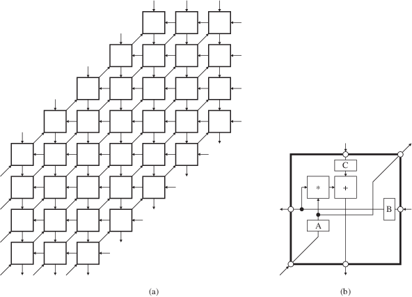
How system (16.3) is related to Figure 16.3? No doubt that you were able to fully understand the operation of the systolic array from Section 16.1 without any special aid. But for the present example this is considerably more difficult—so now you may be sufficiently motivated for the use of a mathematical formalism.
We can assign two fundamental measures to each elementary operation of an algorithm for describing the execution in the systolic array: the time when the operation is performed, and the position of the cell where the operation is performed. As will become clear in the sequel, after fixing the so-called space-time transformation there are hardly any degrees of freedom left for further design: practically all features of the intended systolic array strictly follow from the chosen space-time transformation.
As for the systolic array from Figure 16.1, the execution of an instance  in the systolic array from Figure 16.3 happens at time
  . We can represent this expression as the dot product of a time vector

by the iteration vector

hence

so in this case
The space coordinates  of the executed operations in the example from Figure 16.1 can be inferred as
  from the iteration vector
  according to our decision in Subsection 16.1.3. The chosen map is a projection of the space
  along the
  axis. This linear map can be described by a projection matrix

To find the space coordinates, we multiply the projection matrix  by the iteration vector
  , written as

The projection direction can be represented by any vector  perpendicular to all rows of the projection matrix,

For the projection matrix  from (16.8), one of the possible projection vectors would be
  .
.
Projections are very popular for describing the space coordinates when designing a systolic array. Also in our example from Figure 16.3(a), the space coordinates are generated by projecting the iteration vector. Here, a feasible projection matrix is given by

A corresponding projection vector would be  .
.
We can combine the projection matrix and the time vector in a matrix  , that fully describes the space-time transformation,

The first and second rows of  are constituted by the projection matrix
  , the third row by the time vector
  .
.
For the example from Figure 16.1, the matrix  giving the space-time transformation reads as
for the example from Figure 16.3 we have
Space-time transformations may be understood as a global view to the systolic system. Applying a space-time transformation—that is linear, here, and described by a matrix  —to a system of recurrence equations directly yields the external features of the systolic array, i.e., its architecture—consisting of space coordinates, connection pattern, and cell structure.
Remark. Instead of purely linear maps, we alternatively may consider general affine maps, additionally providing a translative component,  . Though as long as we treat all iteration vectors with a common space-time transformation, affine maps are not really required.
If the domains are numerically given and contain few points in particular, we can easily calculate the concrete set of space coordinates via equation (16.9). But when the domains are specified parametrically as in system (16.3), the positions of the cells must be determined by symbolic evaluation. The following explanation especially dwells on this problem.
Suppose that each cell of the systolic array is represented geometrically by a point with space coordinates  in the two-dimensional space
  . From each iteration vector
  of the domain
  , by equation (16.9) we get the space coordinates
  of a certain processor,
  : the operations denoted by
  are projected onto cell
  . The set
  of space coordinates states the positions of all cells in the systolic array necessary for correct operation.
To our advantage, we normally use domains that can be described as the set of all integer points inside a convex region, here a subset of  —called dense convex domains. The convex hull of such a domain with a finite number of domain points is a polytope, with domain points as vertices. Polytopes map to polytopes again by arbitrary linear transformations. Now we can make use of the fact that each projection is a linear transformation. Vertices of the destination polytope then are images of vertices of the source polytope.
Remark. But not all vertices of a source polytope need to be projected to vertices of the destination polytope, see for instance Figure 16.4.
Figure 16.4. Image of a rectangular domain under projection. Most interior points have been suppressed for clarity. Images of previous vertex points are shaded.
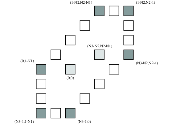
When projected by an integer matrix  , the lattice
  maps to the lattice
  if
if  can be extended by an integer time vector
  to a unimodular space-time matrix
  . Practically any dense convex domain, apart from some exceptions irrelevant to usual applications, thereby maps to another dense convex set of space coordinates, that is completely characterised by the vertices of the hull polytope. To determine the shape and the size of the systolic array, it is therefore sufficient to apply the matrix
  to the vertices of the convex hull of
  .
.
Remark. Any square integer matrix with determinant  is called unimodular. Unimodular matrices have unimodular inverses.
We apply this method to the integer domain

from system (16.3). The vertices of the convex hull here are

For the projection matrix  from (16.11), the vertices of the corresponding image have the positions

Since  has eight vertices, but the image
  only six, it is obvious that two vertices of
  have become interior points of the image, and thus are of no relevance for the size of the array; namely the vertices
  and
and  . This phenomenon is sketched in Figure 16.4.
The settings  ,
,  , and
, and  yield the vertices (3,0), (3,-2), (0,-2), (-4,2), (-4,4), and (-1,4). We see that space coordinates in principle can be negative. Moreover, the choice of an origin—that here lies in the interior of the polytope—might not always be obvious.
As the image of the projection, we get a systolic array with hexagonal shape and parallel opposite borders. On these, we find  ,
,  , and
, and  integer points, respectively; cf. Figure 16.5. Thus, as opposed to our first example, all problem parameters here are also array parameters.
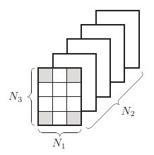
The area function of this region is of order  , and thus depends on all three matrix dimensions. So this is quite different from the situation in Figure 16.1(a), where the area function—for the same problem—is of order
  .
.
Improving on this approximate calculation, we finally count the exact number of cells. For this process, it might be helpful to partition the entire region into subregions for which the number of cells comprised can be easily determined; see Figure 16.5. The points (0,0),  ,
,  , and
, and  are the vertices of a rectangle with
  cells. If we translate this point set up by
  cells and right by
  cells, we exactly cover the whole region. Each shift by one cell up and right contributes just another
  cells. Altogether this yields
  cells.
For  ,
,  , and
, and  we thereby get a number of 36 cells, as we have already learned from Figure 16.3(a).
The running time of a systolic algorithm can be symbolically calculated by an approach similar to that in Subsection 16.2.3. The time transformation according to formula (16.6) as well is a linear map. We find the timesteps of the first and the last calculations as the minimum resp. maximum in the set  of execution timesteps. Following the discussion above, it thereby suffices to vary
  over the vertices of the convex hull of
  .
.
The running time is then given by the formula

Adding one is mandatory here, since the first as well as the last timestep belong to the calculation.
For the example from Figure 16.3, the vertices of the polytope as enumerated in (16.16) are mapped by (16.7) to the set of images

With the basic assumption  , we get a minimum of 3 and a maximum of
  , thus a running time of
  timesteps, as for the systolic array from Figure 16.1—no surprise, since the domains and the time vectors agree.
For the special problem parameters  ,
,  , and
, and  , a running time of
  timesteps can be derived.
If  , the systolic algorithm shows a running time of order
  , using
  systolic cells.
The communication topology of the systolic array is induced by applying the space-time transformation to the data dependences of the algorithm. Each data dependence results from a direct use of a variable instance to calculate another instance of the same variable, or an instance of another variable.
Remark. In contrast to the general situation where a data dependence analysis for imperative programming languages has to be performed by highly optimising compilers, data dependences here always are flow dependences. This is a direct consequence from the assignment-free notation employed by us.
The data dependences can be read off the quantified equations in our assignment-free notation by comparing their right and left sides. For example, we first analyse the equation  from system (16.3).
The value  is calculated from the values
  ,
,  , and
, and  . Thus we have a data flow from
  to
to  , a data flow from
  to
to  , and a data flow from
  to
to  .
.
All properties of such a data flow that matter here can be covered by a dependence vector, which is the iteration vector of the calculated variable instance minus the iteration vector of the correspondingly used variable instance.
The iteration vector for  is
is  ; that for
  is
is  . Thus, as the difference vector, we find

Correspondingly, we get
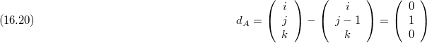
and

In the equation  from system (16.3), we cannot directly recognise which is the calculated variable instance, and which is the used variable instance. This example elucidates the difference between equations and assignments. When fixing that
  should follow from
  by a copy operation, we get the same dependence vector
  as in (16.20). Correspondingly for the equation
  .
.
A variable instance with iteration vector  is calculated in cell
  . If for this calculation another variable instance with iteration vector
  is needed, implying a data dependence with dependence vector
  , the used variable instance is provided by cell
  . Therefore, we need a communication from cell
  to cell
  . In systolic arrays, all communication has to be via direct static links between the communicating cells. Due to the linearity of the transformation from (16.9), we have
  .
.
If  , communication happens exclusively inside the calculating cell, i.e., in time, only—and not in space. Passing values in time is via registers of the calculating cell.
Whereas for  , a communication between different cells is needed. Then a link along the flow direction
  must be provided from/to all cells of the systolic array. The vector
  , oriented in counter flow direction, leads from space point
  to space point
  .
.
If there is more than one dependence vector  , we need an appropriate link for each of them at every cell. Take for example the formulas (16.19), (16.20), and (16.21) together with (16.11), then we get
  ,
,  , and
, and  . In Figure 16.3(a), terminating at every cell, we see three links corresponding to the various vectors
  . This results in a hexagonal communication topology—instead of the orthogonal communication topology from the first example.
Now we apply the space-related techniques from Subsection 16.2.5 to time-related questions. A variable instance with iteration vector  is calculated in timestep
  . If this calculation uses another variable instance with iteration vector
  , the former had been calculated in timestep
  . Hence communication corresponding to the dependence vector
  must take exactly
  timesteps.
Since (16.6) describes a linear map, we have  . According to the systolic principle, each communication must involve at least one register. The dependence vectors
  are fixed, and so the choice of a time vector
  is constrained by

In case  , we must provide registers for stationary variables in all cells. But each register is overwritten with a new value in every timestep. Hence, if
  , the old value must be carried on to a further register. Since this is repeated for
  timesteps, the cell needs exactly
  registers per stationary variable. The values of the stationary variable successively pass all these registers before eventually being used. If
  , the transport of values analogously goes by
  registers, though these are not required to belong all to the same cell.
For each dependence vector  , we thus need an appropriate number of registers. In Figure 16.3(b), we see three input ports at the cell, corresponding to the dependence vectors
  ,
,  , and
, and  . Since for these we have
  . Moreover,
  due to (16.7) and (16.4). Thus, we need one register per dependence vector. Finally, the regularity of system (16.3) forces three output ports for every cell, opposite to the corresponding input ports.
Good news: we can infer in general that each cell needs only a few registers, because the number of dependence vectors  is statically bounded with a system like (16.3), and for each of the dependence vectors the amount of registers
  has a fixed and usually small value.
The three input and output ports at every cell now permit the use of three moving matrices. Very differently from Figure 16.1, a dot product  here is not calculated within a single cell, but dispersed over the systolic array. As a prerequisite, we had to dissolve the sum into a sequence of single additions. We call this principle a distributed generic operator.
Apart from the three input ports with their registers, and the three output ports, Figure 16.3(b) shows a multiplier chained to an adder. Both units are induced in each cell by applying the transformation (16.9) to the domain  of the equation
  from system (16.3). According to this equation, the addition has to follow the calculation of the product, so the order of the hardware operators as seen in Figure 16.3(b) is implied.
The source cell for each of the used operands follows from the projection of the corresponding dependence vector. Here, variable  is related to the dependence vector
  . The projection
  constitutes the flow direction of matrix
  . Thus the value to be used has to be expected, as observed by the calculating cell, in opposite direction
  , in this case from the port in the lower left corner of the cell, passing through register A. All the same,
  comes from the right via register B, and
  from above through register C. The calculated values
  ,
,  , and
, and  are output into the opposite directions through the appropriate ports: to the upper right, to the left, and downwards.
If alternatively we use the projection matrix  from (16.8), then for
  we get the direction
  . The formula
  results in the requirement of exactly one register C for each item of the matrix
  . This register provides the value
  for the calculation of
  , and after this calculation receives the value
  . All this reasoning matches with the cell from Figure 16.1(b). Figure 16.1(a) correspondingly shows no links for matrix
  between the cells: for the matrix is stationary.
Exercises
16.2-1 Each projection vector  induces several corresponding projection matrices
  .
.
-
a. Show that
also is a projection matrix fitting with projection vector
 .
. -
b. Use this projection matrix to transform the domain from system (16.3).
-
c. The resulting space coordinates differ from that in Subsection 16.2.3. Why, in spite of this, both point sets are topologically equivalent?
-
d. Analyse the cells in both arrangements for common and differing features.
16.2-2 Apply all techniques from Section 16.2 to system (16.3), employing a space-time matrix
In Figure 16.3(a), the input/output scheme is only sketched by the flow directions for the matrices  . The necessary details to understand the input/output operations are now provided by Figure 16.6.
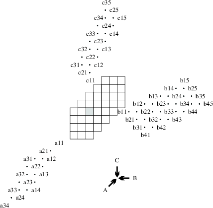
The input/output scheme in Figure 16.6 shows some new phenomena when compared with Figure 16.1(a). The input and output cells belonging to any matrix are no longer threaded all on a single straight line; now, for each matrix, they lie along two adjacent borders, that additionally may differ in the number of links to the outside world. The data structures from Figure 16.6 also differ from that in Figure 16.1(a) in the angle of inclination. Moreover, the matrices  and
and  from Figure 16.6 arrive at the boundary cells with only one third of the data rate, compared to Figure 16.1(a).
Spending some effort, even here it might be possible in principle to construct—item by item—the appropriate input/output scheme fitting the present systolic array. But it is much more safe to apply a formal derivation. The following subsections are devoted to the presentation of the various methodical steps for achieving our goal.
First, we need to construct a formal relation between the abstract data structures and the concrete variable instances in the assignment-free representation.
Each item of the matrix  can be characterised by a row index
  and a column index
  . These data structure indices can be comprised in a data structure vector
  . Item
  in system (16.3) corresponds to the instances
  , with any
  . The coordinates of these instances all lie on a line along direction
  in space
  . Thus, in this case, the formal change from data structure vector
  to coordinates
  can be described by the transformation

In system (16.3), the coordinate vector  of every variable instance equals the iteration vector of the domain point representing the calculation of this variable instance. Thus we also may interpret formula (16.23) as a relation between data structure vectors and iteration vectors. Abstractly, the desired iteration vectors
  can be inferred from the data structure vector
  by the formula

The affine vector  is necessary in more general cases, though always null in our example.
Because of  , the representation for matrix
  correspondingly is

Concerning matrix  , each variable instance
  may denote a different value. Nevertheless, all instances
  to a fixed index pair
  can be regarded as belonging to the same matrix item
  , since they all stem from the serialisation of the sum operator for the calculation of
  . Thus, for matrix
  , following formula (16.24) we may set

Each of the three matrices  is generated by two directions with regard to the data structure indices: along a row, and along a column. The difference vector (0,1) thereby describes a move from an item to the next item of the same row, i.e., in the next column:
  . Correspondingly, the difference vector (1,0) stands for sliding from an item to the next item in the same column and next row:
  .
.
Input/output schemes of the appearance shown in Figures 16.1(a) and 16.6 denote snapshots: all positions of data items depicted, with respect to the entire systolic array, are related to a common timestep.
As we can notice from Figure 16.6, the rectangular shapes of the abstract data structures are mapped to parallelograms in the snapshot, due to the linearity of the applied space-time transformation. These parallelograms can be described by difference vectors along their borders, too.
Next we will translate difference vectors  from data structure vectors into spatial difference vectors
  for the snapshot. Therefore, by choosing the parameter
  in formula (16.24), we pick a pair of iteration vectors
  that are mapped to the same timestep under our space-time transformation. For the moment it is not important which concrete timestep we thereby get. Thus, we set up

implying

and thus

Due to the linearity of all used transformations, the wanted spatial difference vector  hence follows from the difference vector of the data structure
  as
as

or

With the aid of formula (16.31), we now can determine the spatial difference vectors  for matrix
  . As mentioned above, we have
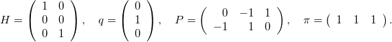
Noting  , we get

For the rows, we have the difference vector  , yielding the spatial difference vector
  . Correspondingly, from
  for the columns we get
  . If we check with Figure 16.6, we see that the rows of
  in fact run along the vector
  , the columns along the vector
  .
.
Similarly, we get  for the rows of
  , and
, and  for the columns of
  ; as well as
  for the rows of
  , and
, and 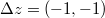 for the columns of
  .
.
Applying these instruments, we are now able to reliably generate appropriate input/output schemes—although separately for each matrix at the moment.
Now, the shapes of the matrices  for the snapshot have been fixed. But we still have to adjust the matrices relative to the systolic array—and thus, also relative to each other. Fortunately, there is a simple graphical method for doing the task.
We first choose an arbitrary iteration vector, say  . The latter we map with the projection matrix
  to the cell where the calculation takes place,
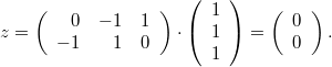
The iteration vector (1,1,1) represents the calculations  ,
,  , and
, and  ; these in turn correspond to the data items
  ,
,  , and
, and  . We now lay the input/output schemes for the matrices
  on the systolic array in a way that the entries
  ,
,  , and
, and  all are located in cell
  .
.
In principle, we would be done now. Unfortunately, our input/output schemes overlap with the cells of the systolic array, and are therefore not easily perceivable. Thus, we simultaneously retract the input/output schemes of all matrices in counter flow direction, place by place, until there is no more overlapping. With this method, we get exactly the input/output scheme from Figure 16.6.
As an alternative to this nice graphical method, we also could formally calculate an overlap-free placement of the various input/output schemes.
Only after specifying the input/output schemes, we can correctly calculate the number of timesteps effectively needed. The first relevant timestep starts with the first input operation. The last relevant timestep ends with the last output of a result. For the example, we determine from Figure 16.6 the beginning of the calculation with the input of the data item  in timestep 0, and the end of the calculation after output of the result
  in timestep 14. Altogether, we identify 15 timesteps—five more than with pure treatment of the real calculations.
The input schemes of the matrices  and
and  from Figure 16.1(a) have a dense layout: if we drew the borders of the matrices shown in the figure, there would be no spare places comprised.
Not so in Figure 16.6. In any input data stream, each data item is followed by two spare places there. For the input matrices this means: the boundary cells of the systolic array receive a proper data item only every third timestep.
This property is a direct result of the employed space-time transformation. In both examples, the abstract data structures themselves are dense. But how close the various items really come in the input/output scheme depends on the absolute value of the determinant of the transformation matrix  : in every input/output data stream, the proper items follow each other with a spacing of exactly
  places. Indeed
  for Figure 16.1; as for Figure 16.6, we now can rate the fluffy spacing as a practical consequence of
  .
.
What to do with spare places as those in Figure 16.6? Although each cell of the systolic array from Figure 16.3 in fact does useful work only every third timestep, it would be nonsense to pause during two out of three timesteps. Strictly speaking, we can argue that values on places marked with dots in Figure 16.6 have no influence on the calculation of the shown items  , because they never reach an active cell at time of the calculation of a variable
  . Thus, we may simply fill spare places with any value, no danger of disturbing the result. It is even feasible to execute three different matrix products at the same time on the systolic array from Figure 16.3, without interference. This will be our topic in Subsection 16.3.7.
When further studying Figure 16.6, we can identify another problem. Check, for example, the itinerary of  through the cells of the systolic array. According to the space-time transformation, the calculations contributing to the value of
  happen in the cells
  ,
,  ,
,  , and
, and  . But the input/output scheme from Figure 16.6 tells us that
  also passes through cell
  before, and eventually visits cell
  , too.
This may be interpreted as some spurious calculations being introduced into the system (16.3) by the used space-time transformation, here, for example, at the new domain points (2,2,0) and (2,2,5). The reason for this phenomenon is that the domains of the input/output operations are not in parallel to the chosen projection direction. Thus, some input/output operations are projected onto cells that do not belong to the boundary of the systolic array. But in the interior of the systolic array, no input/output operation can be performed directly. The problem can be solved by extending the trajectory, in flow or counter flow direction, from these inner cells up to the boundary of the systolic array. But thereby we introduce some new calculations, and possibly also some new domain points. This technique is called input/output expansion.
We must avoid that the additional calculations taking place in the cells (-2,0) and (3,0) corrupt the correct value of  . For the matrix product, this is quite easy—though the general case is more difficult. The generic sum operator has a neutral element, namely zero. Thus, if we can guarantee that by new calculations only zero is added, there will be no harm. All we have to do is providing always at least one zero operand to any spurious multiplication; this can be achieved by filling appropriate input slots with zero items.
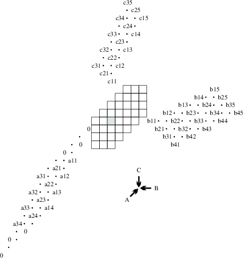
Figure 16.7 shows an example of a properly extended input/output scheme. Preceding and following the items of matrix  , the necessary zero items have been filled in. Since the entered zeroes count like data items, the input/output scheme from Figure 16.6 has been retracted again by one place. The calculation now begins already in timestep
  , but ends as before with timestep 14. Thus we need 16 timesteps altogether.
Let us come back to the example from Figure 16.1(a). For inputting the items of matrices  and
and  , no expansion is required, since these items are always used in boundary cells first. But not so with matrix
  ! The items of
  are calculated in stationary variables, hence always in the same cell. Thus most results
  are produced in inner cells of the systolic array, from where they have to be moved—in a separate action—to boundary cells of the systolic array.
Although this new challenge, on the face of it, appears very similar to the problem from Subsection 16.3.5, and thus very easy to solve, in fact we here have a completely different situation. It is not sufficient to extend existing data flows forward or backward up to the boundary of the systolic array. Since for stationary variables the dependence vector is projected to the null vector, which constitutes no extensible direction, there can be no spatial flow induced by this dependency. Possibly, we can construct some auxiliary extraction paths, but usually there are many degrees of freedom. Moreover, we then need a control mechanism inside the cells. For all these reasons, the problem is further dwelled on in Section 16.4.
As can be easily noticed, the utilisation of the systolic array from Figure 16.3 with input/output scheme from Figure 16.7 is quite poor. Even without any deeper study of the starting phase and the closing phase, we cannot ignore that the average utilisation of the array is below one third—after all, each cell at most in every third timestep makes a proper contribution to the calculation.
A simple technique to improve this behaviour is to interleave calculations. If we have three independent matrix products, we can successively input their respective data, delayed by only one timestep, without any changes to the systolic array or its cells. Figure 16.8 shows a snapshot of the systolic array, with parts of the corresponding input/output scheme. Now we must check by a formal derivation whether this idea is really working. Therefore, we slightly modify system (16.3). We augment the variables and the domains by a fourth dimension, needed to distinguish the three matrix products:
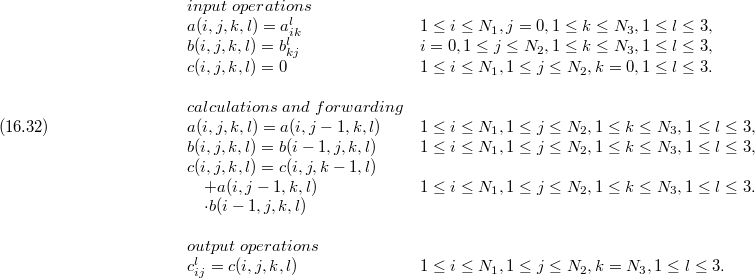
Figure 16.8. Interleaved calculation of three matrix products on the systolic array from Figure 16.3.
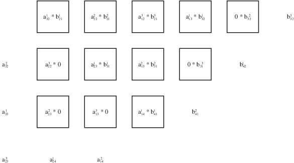
Obviously, in system (16.32), problems with different values of  are not related. Now we must preserve this property in the systolic array. A suitable space-time matrix would be
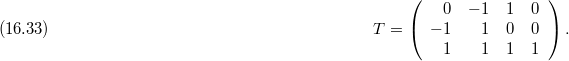
Notice that  is not square here. But for calculating the space coordinates, the fourth dimension of the iteration vector is completely irrelevant, and thus can simply be neutralised by corresponding zero entries in the fourth column of the first and second rows of
  .
.
The last row of  again constitutes the time vector
  . Appropriate choice of
  embeds the three problems to solve into the space-time continuum, avoiding any intersection. Corresponding instances of the iteration vectors of the three problems are projected to the same cell with a respective spacing of one timestep, because the fourth entry of
  equals 1.
Finally, we calculate the average utilisation—with or without interleaving—for the concrete problem parameters  ,
,  , and
, and  . For a single matrix product, we have to perform
  calculations, considering a multiplication and a corresponding addition as a compound operation, i.e., counting both together as only one calculation; input/output operations are not counted at all. The systolic array has 36 cells.
Without interleaving, our systolic array altogether takes 16 timesteps for calculating a single matrix product, resulting in an average utilisation of  calculations per timestep and cell. When applying the described interleaving technique, the calculation of all three matrix products needs only two timesteps more, i.e., 18 timesteps altogether. But the number of calculations performed thereby has tripled, so we get an average utilisation of the cells amounting to
  calculations per timestep and cell. Thus, by interleaving, we were able to improve the utilisation of the cells to 267 per cent!
Exercises
16.3-1 From equation (16.31), formally derive the spatial difference vectors of matrices  and
and  for the input/output scheme shown in Figure 16.6.
16.3-2 Augmenting Figure 16.6, draw an extended input/output scheme that forces both operands of all spurious multiplications to zero.
16.3-3 Apply the techniques presented in Section 16.3 to the systolic array from Figure 16.1.
16.3-4 Proof the properties claimed in Subsection 16.3.7 for the special space-time transformation (16.33) with respect to system (16.32).
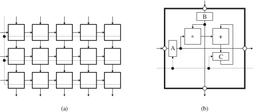
So far we have assumed that each cell of a systolic array behaves in completely the same way during every timestep. Admittedly there are some relevant examples of such systolic arrays. However, in general the cells successively have to work in several operation modes, switched to by some control mechanism. In the sequel, we study some typical situations for exerting control.
The cell from Figure 16.3(b) contains the registers A, B, and C, that—when activated by the global clock signal—accept the data applied to their inputs and then reliably reproduce these values at their outputs for one clock cycle. Apart from this system-wide activity, the function calculated by the cell is invariant for all timesteps: a fused multiply-add operation is applied to the three input operands  ,
,  , and
, and  , with result passed to a neighbouring cell; during the same cycle, the operands
  and
and  are also forwarded to two other neighbouring cells. So in this case, the cell needs no control at all.
The initial values  for the execution of the generic sum operator—which could also be different from zero here—are provided to the systolic array via the input streams, see Figure 16.7; the final results
  continue to flow into the same direction up to the boundary of the array. Therefore, the input/output activities for the cell from Figure 16.3(b) constitute an intrinsic part of the normal cell function. The price to pay for this extremely simple cell function without any control is a restriction in all three dimensions of the matrices: on a systolic array like that from Figure 16.3, with fixed array parameters
  , an
, an  matrix
  can only be multiplied by an
  matrix
  if the relations
  ,
,  , and
, and  hold.
hold.
In this respect, constraints for the array from Figure 16.1 are not so restrictive: though the problem parameters  and
and  also are bounded by
  and
and  , there is no constraint for
  . Problem parameters unconstrained in spite of fixed array parameters can only emerge in time but not in space, thus mandating the use of stationary variables.
Before a new calculation can start, each register assigned to a stationary variable has to be reset to an initial state independent from the previously performed calculations. For instance, concerning the systolic cell from Figure 16.3(b), this should be the case for register C. By a global signal similar to the clock, register C can be cleared in all cells at the same time, i.e., reset to a zero value. To prevent a corruption of the reset by the current values of A or B, at least one of the registers A or B must be cleared at the same time, too. Figure 16.9 shows an array structure and a cell structure implementing this idea.
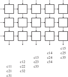
Unfortunately, for the matrix product the principle of the global control is not sufficient without further measures. Since the systolic array presented in Figure 16.1 even lacks another essential property: the results  are not passed to the boundary but stay in the cells.
At first sight, it seems quite simple to forward the results to the boundary: when the calculation of an item  is finished, the links from cell
  to the neighbouring cells
  and
and  are no longer needed to forward items of the matrices
  and
and  . These links can be reused then for any other purpose. For example, we could pass all items of
  through the downward-directed links to the lower border of the systolic array.
But it turns out that leading through results from the upper cells is hampered by ongoing calculations in the lower parts of the array. If the result  , finished in timestep
  , would be passed to cell
  in the next timestep, a conflict would be introduced between two values: since only one value per timestep can be sent from cell
  via the lower port, we would be forced to keep either
  or
or  , the result currently finished in cell
  . This effect would spread over all cells down.
To fix the problem, we could slow down the forwarding of items  . If it would take two timesteps for
  to pass a cell, no collisions could occur. Then, the results stage a procession through the same link, each separated from the next by one timestep. From the lower boundary cell of a column, the host computer first receives the result of the bottom row, then that of the penultimate row; this procedure continues until eventually we see the result of the top row. Thus we get the output scheme shown in Figure 16.10.
How can a cell recognise when to change from forwarding items of matrix  to passing items of matrix
  through the lower port? We can solve this task by an automaton combining global control with local control in the cell:
If we send a global signal to all cells at exactly the moment when the last items of  and
and  are input to cell
  , each cell can start a countdown process: in each successive timestep, we decrement a counter initially set to the number of the remaining calculation steps. Thereby cell
  still has to perform
  calculations before changing to propagation mode. Later, the already mentioned global reset signal switches the cell back to calculation mode.
Figure 16.11 presents a systolic array implementing this local/global principle. Basically, the array structure and the communication topology have been preserved. But each cell can run in one of two states now, switched by a control logic:
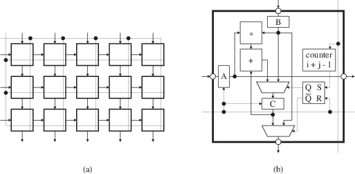
-
In calculation mode, as before, the result of the addition is written to register C. At the same time, the value in register B—i.e., the operand used for the multiplication—is forwarded through the lower port of the cell.
-
In propagation mode, registers B and C are connected in series. In this mode, the only function of the cell is to guide each value received at the upper port down to the lower port, thereby enforcing a delay of two timesteps.
The first value output from cell  in propagation mode is the currently calculated value
  , stored in register C. All further output values are results forwarded from cells above. A formal description of the algorithm implemented in Figure 16.11 is given by the assignment-free system (16.34).
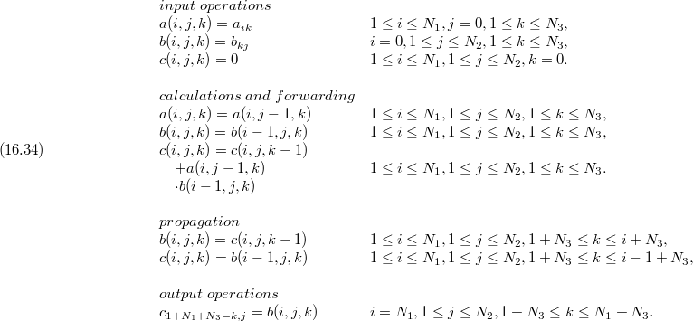
It rests to explain how the control signals in a cell are generated in this model. As a prerequisite, the cell must contain a state flip-flop indicating the current operation mode. The output of this flip-flop is connected to the control inputs of both multiplexors, see Figure 16.11(b). The global reset signal clears the state flip-flop, as well as the registers A and C: the cell now works in calculation mode.
The global ready signal starts the countdown in all cells, so in every timestep the counter is diminished by 1. The counter is initially set to the precalculated value  , dependent on the position of the cell. When the counter reaches zero, the flip-flop is set: the cell switches to propagation mode.
If desisting from a direct reset of the register C, the last value passed, before the reset, from register B to register C of a cell can be used as a freely decidable initial value for the next dot product to evaluate in the cell. We then even calculate, as already in the systolic array from Figure 16.3, the more general problem

detailed by the following equation system:

The method sketched in Figure 16.11 still has the following drawbacks:
-
The systolic array uses global control signals, requiring a high technical accuracy.
-
Each cell needs a counter with counting register, introducing a considerable hardware expense.
-
The initial value of the counter varies between the cells. Thus, each cell must be individually designed and implemented.
-
The input data of any successive problem must wait outside the cells until all results from the current problem have left the systolic array.
These disadvantages can be avoided, if control signals are propagated like data—meaning a distributed control. Therefore, we preserve the connections of the registers B and C with the multiplexors from Figure 16.11(b), but do not generate any control signals in the cells; also, there will be no global reset signal. Instead, a cell receives the necessary control signal from one of the neighbours, stores it in a new one-bit register S, and appropriately forwards it to further neighbouring cells. The primary control signals are generated by the host computer, and infused into the systolic array by boundary cells, only. Figure 16.12(a) shows the required array structure, Figure 16.12(b) the modified cell structure.
Switching to the propagation mode occurs successively down one cell in a column, always delayed by one timestep. The delay introduced by register S is therefore sufficient.
Reset to the calculation mode is performed via the same control wire, and thus also happens with a delay of one timestep per cell. But since the results  sink down at half speed, only, we have to wait sufficiently long with the reset: if a cell is switched to calculation mode in timestep
  , it goes to propagation mode in timestep
  , and is reset back to calculation mode in timestep
  .
.
So we learned that in a systolic array, distributed control induces a different macroscopic timing behaviour than local/global control. Whereas the systolic array from Figure 16.12 can start the calculation of a new problem (16.35) every  timesteps, the systolic array from Figure 16.11 must wait for
  timesteps. The time difference
  resp.
resp.  is called the period, its reciprocal being the throughput.
System (16.37 and 16.38), divided into two parts during the typesetting, formally describes the relations between distributed control and calculations. We thereby assume an infinite, densely packed sequence of matrix product problems, the additional iteration variable  being unbounded. The equation headed variables with alias describes but pure identity relations.
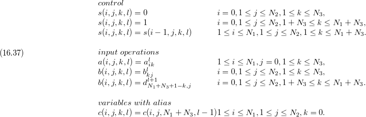
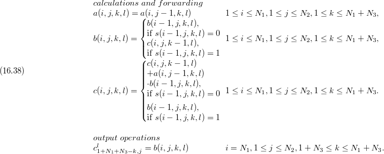
Figure 16.12. Matrix product on a rectangular systolic array, with output of results and distributed control. (a) Array structure. (b) Cell structure.
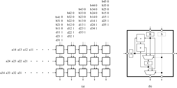
Formula (16.39) shows the corresponding space-time matrix. Note that one entry of  is not constant but depends on the problem parameters:
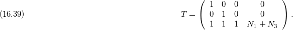
Interestingly, also the cells in a row switch one timestep later when moving one position to the right. Sacrificing some regularity, we could use this circumstance to relieve the host computer by applying control to the systolic array at cell (1,1), only. We therefore would have to change the control scheme in the following way:
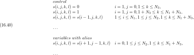
Figure 16.13. Matrix product on a rectangular systolic array, with output of results and distributed control. (a) Array structure. (b) Cell on the upper border.
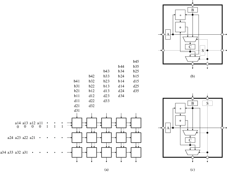
Figure 16.13 shows the result of this modification. We now need cells of two kinds: cells on the upper border of the systolic array must be like that in Figure 16.13(b); all other cells would be as before, see Figure 16.13(c). Moreover, the communication topology on the upper border of the systolic array would be slightly different from that in the regular area.
The chosen space-time transformation widely determines the architecture of the systolic array. Mapping recurrence equations to space-time coordinates yields an explicit view to the geometric properties of the systolic array, but gives no real insight into the function of the cells. In contrast, the processes performed inside a cell can be directly expressed by a cell program. This approach is particularly of interest if dealing with a programmable systolic array, consisting of cells indeed controlled by a repetitive program.
Like the global view, i.e., the structure of the systolic array, the local view given by a cell program in fact is already fixed by the space-time transformation. But, this local view is only induced implicitly here, and thus, by a further mathematical transformation, an explicit representation must be extracted, suitable as a cell program.
In general, we denote instances of program variables with the aid of index expressions, that refer to iteration variables. Take, for instance, the equation

from system (16.3). The instance  of the program variable
  is specified using the index expressions
  ,
,  , and
, and  , which can be regarded as functions of the iteration variables
  .
.
As we have noticed, the set of iteration vectors  from the quantification becomes a set of space-time coordinates
  when applying a space-time transformation (16.12) with transformation matrix
  from (16.14),

Since each cell is denoted by space coordinates  , and the cell program must refer to the current time
  , the iteration variables
  in the index expressions for the program variables are not suitable, and must be translated into the new coordinates
  . Therefore, using the inverse of the space-time transformation from (16.41), we express the iteration variables
  as functions of the space-time coordinates
  ,
,

The existence of such an inverse transformation is guaranteed if the space-time transformation is injective on the domain—and that it should always be: if not, some instances must be calculated by a cell in the same timestep. In the example, reversibility is guaranteed by the square, non singular matrix  , even without referral to the domain. With respect to the time vector
  and any projection vector
  , the property
  is sufficient.
Replacing iteration variables by space-time coordinates, which might be interpreted as a transformation of the domain, frequently yields very unpleasant index expressions. Here, for example, from  we get

But, by a successive transformation of the index sets, we can relabel the instances of the program variables such that the reference to cell and time appears more evident. In particular, it seems worthwhile to transform the equation system back into output normal form, i.e., to denote the results calculated during timestep  in cell
  by instances
  of the program variables. We best gain a real understanding of this approach via an abstract mathematical formalism, that we can fit to our special situation.
Therefore, let

be a quantified equation over a domain  , with program variables
  and
and  . The index functions
  and
and  generate the instances of the program variables as tuples of index expressions.
By transforming the domain with a function  that is injective on
  , equation (16.43) becomes

where  is a function that constitutes an inverse of
  on
on  . The new index functions are
  and
and  . Transformations of index sets don't touch the domain; they can be applied to each program variable separately, since only the instances of this program variable are renamed, and in a consistent way. With such renamings
  and
and  , equation (16.44) becomes

If output normal form is desired,  has to be the identity.
In the most simple case (as for our example),  is the identity, and
  is an affine transformation of the form
 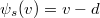 , with constant
  —the already known dependence vector.
  then can be represented in the same way, with
  . Transformation of the domains happens by the space-time transformation
  , with an invertible matrix
  . For all index transformations, we choose the same
  . Thus equation (16.45) becomes

For the generation of a cell program, we have to know the following information for every timestep: the operation to perform, the source of the data, and the destination of the results—known from assembler programs as opc, src, dst.
The operation to perform (opc) follows directly from the function  . For a cell with control, we must also find the timesteps when to perform this individual function
  . The set of these timesteps, as a function of the space coordinates, can be determined by projecting the set
  onto the time axis; for general polyhedric
  with the aid of a Fourier-Motzkin elimination, for example.
In system (16.46), we get a new dependence vector  , consisting of two components: a (vectorial) spatial part, and a (scalar) timely part. The spatial part
  , as a difference vector, specifies which neighbouring cell has calculated the operand. We directly can translate this information, concerning the input of operands to cell
  , into a port specifier with port position
  , serving as the
 src operand of the instruction. In the same way, the cell calculating the operand, with position  , must write this value to a port with port position
  , used as the
 dst operand in the instruction.
The timely part of  specifies, as a time difference
  , when the calculation of the operand has been performed. If
  , this information is irrelevant, because the reading cell
  always gets the output of the immediately preceding timestep from neighbouring cells. However, for
  , the value must be buffered for
  timesteps, either by the producer cell
  , or by the consumer cell
  —or by both, sharing the burden. This need can be realised in the cell program, for example, with
  copy instructions executed by the producer cell
  , preserving the value of the operand until its final output from the cell by passing it through
  registers.
Applying this method to system (16.37 and 16.38), with transformation matrix  as in (16.39), yields
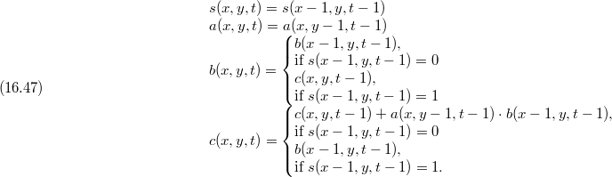
The iteration variable l, being relevant only for the input/output scheme, can be set to a fixed value prior to the transformation. The cell program for the systolic array from Figure 16.12, performed once in every timestep, reads as follows:
Cell-Program
12
3
4
5
6
IF7
THEN8
9
ELSE10

The port specifiers stand for local input/output to/from the cell. For each, a pair of qualifiers is derived from the geometric position of the ports relative to the centre of the cell. Port  is situated on the left border of the cell,
  on the right border;
  is above the centre,
  below. Each port specifier can be augmented by a bit range:
  stands for bit 0 of the port, only;
 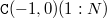 denotes the bits 1 to
  . The designations
  without port qualifiers stand for registers of the cell.
By application of matrix  from (16.13) to system (16.36), we get
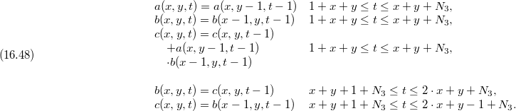
Now the advantages of distributed control become obvious. The cell program for (16.47) can be written with referral to the respective timestep  , only. And thus, we need no reaction to global control signals, no counting register, no counting operations, and no coding of the local cell coordinates.
Exercises
16.4-1 Specify appropriate input/output schemes for performing, on the systolic arrays presented in Figures 16.11 and 16.12, two evaluations of system (16.36) that follow each other closest in time.
16.4-2 How could we change the systolic array from Figure 16.12, to efficiently support the calculation of matrix products with parameters  or
or  ?
?
16.4-3 Write a cell program for the systolic array from Figure 16.3.
16.4-4 Which throughput allows the systolic array from Figure 16.3 for the assumed values of  ? Which for general
  ?
?
16.4-5 Modify the systolic array from Figure 16.1 such that the results stored in stationary variables are output through additional links directed half right down, i.e., from cell  to cell
  . Develop an assignment-free equation system functionally equivalent to system (16.36), that is compatible with the extended structure. How looks the resulting input/output scheme? Which period is obtained?
Figure 16.14. Bubble sort algorithm on a linear systolic array. (a) Array structure with input/output scheme. (b) Cell structure.
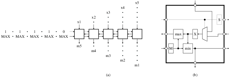
Explanations in the sections above heavily focused on two-dimensional systolic arrays, but in principle also apply to one-dimensional systolic arrays, called linear systolic arrays in the sequel. The most relevant difference between both kinds concerns the boundary of the systolic array. Linear systolic arrays can be regarded as consisting of boundary cells, only; under this assumption, input from and output to the host computer needs no special concern. However, the geometry of a linear systolic array provides one full dimension as well as one fictitious dimension, and thus communication along the full-dimensional axis may involve similar questions as in Subsection 16.3.5. Eventually, the boundary of the linear systolic array can also be defined in a radically different way, namely to consist of both end cells, only.
If we set one of the problem parameters  or
or  to value 1 for a systolic array as that from Figure 16.1, the matrix product means to multiply a matrix by a vector, from left or right. The two-dimensional systolic array then degenerates to a one-dimensional systolic array. The vector by which to multiply is provided as an input data stream through an end cell of the linear systolic array. The matrix items are input to the array simultaneously, using the complete broadside.
As for full matrix product, results emerge stationary. But now, they either can be drained along the array to one of the end cells, or they are sent directly from the producer cells to the host computer. Both methods result in different control mechanisms, time schemes, and running time.
Now, would it be possible to provide all inputs via end cells? The answer is negative if the running time should be of complexity  . Matrix
  contains
  items, thus there are
  items per timestep to read. But the number of items receivable through an end cell during one timestep is bounded. Thus, the input/output data rate—of order
  , here—may already constrain the possible design space.
For sorting, the task is to bring the elements from a set  , subset of a totally ordered basic set
  , into an ascending order
  where
where  for
for  . A solution to this problem is described by the following assignment-free equation system, where
  denotes the maximum in
  :
:
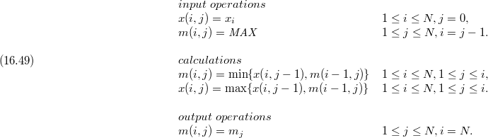
By completing a projection along direction  to a space-time transformation

we get the linear systolic array from Figure 16.14, as an implementation of the bubble sort algorithm.
Correspondingly, the space-time matrix

would induce another linear systolic array, that implements insertion sort. Eventually, the space-time matrix

would lead to still another linear systolic array, this one for selection sort.
For the sorting problem, we have  input items,
  output items, and
  timesteps. This results in an input/output data rate of order
  . In contrast to the matrix-vector product from Subsection 16.5.1, the sorting problem with any prescribed input/output data rate in principle allows to perform the communication exclusively through the end cells of a linear systolic array.
Note that, in all three variants of sorting described so far, direct input is necessary to all cells: the values to order for bubble sort, the constant values  for insertion sort, and both for selection sort. However, instead of inputting the constants, the cells could generate them, or read them from a local memory.
All three variants require a cell control: insertion sort and selection sort use stationary variables; bubble sort has to switch between the processing of input data and the output of calculated values.
System (16.53) below describes a localised algorithm for solving the linear equation system  , where the
  matrix
  is a lower triangular matrix.
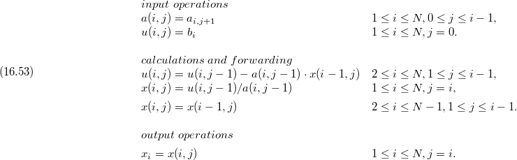
All previous examples had in common that, apart from copy operations, the same kind of calculation had to be performed for each domain point: fused multiply/add for the matrix algorithms, minimum and maximum for the sorting algorithms. In contrast, system (16.53) contains some domain points where multiply and subtract is required, as well as some others needing division. When projecting system (16.53) to a linear systolic array, depending on the chosen projection direction we get fixed or varying cell functions. Peculiar for projecting along  , we see a single cell with divider; all other cells need a multiply/subtract unit. Projection along
  or
or  yields identical cells, all containing a divider as well as a multiply/subtract unit. Projection vector
  results in a linear systolic array with three different cell types: both end cells need a divider, only; all other cells contain a multiply/subtract unit, with or without divider, alternatingly. Thus, a certain projection can introduce inhomogeneities into a systolic array—that may be desirable, or not.
Exercises
16.5-1 For both variants of matrix-vector product as in Subsection 16.5.1—output of the results by an end cell versus communication by all cells—specify a suitable array structure with input/output scheme and cell structure, including the necessary control mechanisms.
16.5-2 Study the effects of further projection directions on system (16.53).
16.5-3 Construct systolic arrays implementing insertion sort and selection sort, as mentioned in Subsection 16.5.2. Also draw the corresponding cell structures.
16.5-4 The systolic array for bubble sort from Figure 16.14 could be operated without control by cleverly organising the input streams. Can you find the trick?
16.5-5 What purpose serves the value  in system (16.49)? How system (16.49) could be formulated without this constant value? Which consequences this would incur for the systolic arrays described?
PROBLEMS |
16-1 Band matrix algorithms
In Sections 16.1, 16.2, and Subsections 16.5.1, and 16.5.3, we always assumed full input matrices, i.e., each matrix item  used could be nonzero in principle. (Though in a lower triangular matrix, items above the main diagonal are all zero. Note, however, that these items are not inputs to any of the algorithms described.)
In contrast, practical problems frequently involve band matrices, cf. Kung/Leiserson [207]. In such a matrix, most diagonals are zero, left alone a small band around the main diagonal. Formally, we have  for all
  with
with  or
or  , where
  and
and  are positive integers. The band width, i.e., the number of diagonals where nonzero items may appear, here amounts to
  .
.
Now the question arises whether we could profit from the band structure in one or more input matrices to optimise the systolic calculation. One opportunity would be to delete cells doing no useful work. Other benefits could be shorter input/output data streams, reduced running time, or higher throughput.
Study all systolic arrays presented in this chapter for improvements with respect to these criteria.
CHAPTER NOTES |
The term systolic array has been coined by Kung and Leiserson in their seminal paper [207].
Karp, Miller, and Winograd did some pioneering work [190] for uniform recurrence equations.
Essential stimuli for a theory on the systematic design of systolic arrays have been Rao's PhD dissertation [282] and the work of Quinton [281].
The contribution of Teich and Thiele [319] shows that a formal derivation of the cell control can be achieved by methods very similar to those for a determination of the geometric array structure and the basic cell function.
The up-to-date book by Darte, Robert, and Vivien [79] joins advanced methods from compiler design and systolic array design, dealing also with the analysis of data dependences.
The monograph [358] still seems to be the most comprehensive work on systolic systems.
Each systolic array can also be modelled as a cellular automaton. The registers in a cell together hold the state of the cell. Thus, a factorised state space is adequate. Cells of different kind, for instance with varying cell functionality or position-dependent cell control, can be described with the aid of further components of the state space.
Each systolic algorithm also can be regarded as a PRAM algorithm with the same timing behaviour. Thereby, each register in a systolic cell corresponds to a PRAM memory cell, and vice versa. The EREW PRAM model is sufficient, because in every timestep exactly one systolic cell reads from this register, and then exactly one systolic cell writes to this register.
Each systolic system also is a special kind of synchronous network as defined by Lynch [228]. Time complexity measures agree. Communication complexity usually is no topic with systolic arrays. Restriction to input/output through boundary cells, frequently demanded for systolic arrays, also can be modelled in a synchronous network. The concept of failures is not required for systolic arrays.
The book written by Sima, Fountain and Kacsuk [304] considers the systolic systems in details.
Table of Contents
- 5. Memory Management
- 6. Relational Database Design
- 7. Query Rewriting in Relational Databases
- 8. Semi-structured Databases
Table of Contents
The main task of computers is to execute programs (even usually several programs running simultaneously). These programs and their data must be in the main memory of the computer during the execution.
Since the main memory is usually too small to store all these data and programs, modern computer systems have a secondary storage too for the provisional storage of the data and programs.
In this chapter the basic algorithms of memory management will be covered. In Section 17.1 static and dynamic partitioning, while in Section 17.2 the most popular paging methods will be discussed.
In Section 17.3 the most famous anomaly of the history of operating systems— the stunning features of FIFO page changing algorithm, interleaved memory and processing algorithms with lists—will be analysed.
Finally in Section 17.4 the discussion of the optimal and approximation algorithms for the optimisation problem in which there are files with given size to be stored on the least number of disks can be found.
A simple way of sharing the memory between programs is to divide the whole address space into slices, and assign such a slice to every process. These slices are called partitions. The solution does not require any special hardware support, the only thing needed is that programs should be ready to be loaded to different memory addresses, i.e., they should be relocatable. This must be required since it cannot be guaranteed that a program always gets into the same partition, because the total size of the executable programs is usually much more than the size of the whole memory. Furthermore, we cannot determine which programs can run simultaneously and which not, for processes are generally independent of each other, and in many cases their owners are different users. Therefore, it is also possible that the same program is executed by different users at the same time, and different instances work with different data, which can therefore not be stored in the same part of the memory. Relocation can be easily performed if the linker does not work with absolute but with relative memory addresses, which means it does not use exact addresses in the memory but a base address and an offset. This method is called base addressing, where the initial address is stored in the so called base register. Most processors know this addressing method, therefore, the program will not be slower than in the case using absolute addresses. By using base addressing it can also be avoided that—due to an error or the intentional behaviour of a user—the program reads or modifies the data of other programs stored at lower addresses of the memory. If the solution is extended by another register, the so called limit register which stores the biggest allowed offset, i.e. the size of the partition, then it can be assured that the program cannot access other programs stored at higher memory addresses either.
Partitioning was often used in mainframe computer operating systems before. Most of the modern operating systems, however, use virtual memory management which requires special hardware support.
Partitioning as a memory sharing method is not only applicable in operating systems. When writing a program in a language close to machine code, it can happen that different data structures with variable size—which are created and cancelled dynamically—have to be placed into a continuous memory space. These data structures are similar to processes, with the exception that security problems like addressing outside their own area do not have to be dealt with. Therefore, most of the algorithms listed below with some minor modifications can be useful for application development as well.
Basically, there are two ways of dividing the address space into partitions. One of them divides the initially empty memory area into slices, the number and size of which is predetermined at the beginning, and try to place the processes and other data structures continuously into them, or remove them from the partitions if they are not needed any more. These are called fixed partitions, since both their place and size have been fixed previously, when starting the operating system or the application. The other method is to allocate slices from the free parts of the memory to the newly created processes and data structures continuously, and to deallocate the slices again when those end. This solution is called dynamic partitioning, since partitions are created and destroyed dynamically. Both methods have got advantages as well as disadvantages, and their implementations require totally different algorithms. These will be discussed in the following.
Using fixed partitions the division of the address space is fixed at the beginning, and cannot be changed later while the system is up. In the case of operating systems the operator defines the partition table which is activated at next reboot. Before execution of the first application, the address space is already partitioned. In the case of applications partitioning has to be done before creation of the first data structure in the designated memory space. After that data structures of different sizes can be placed into these partitions.
In the following we examine only the case of operating systems, while we leave to the Reader the rewriting of the problem and the algorithms according to given applications, since these can differ significantly depending on the kind of the applications.
The partitioning of the address space must be done after examination of the sizes and number of possible processes running on the system. Obviously, there is a maximum size, and programs exceeding it cannot be executed. The size of the largest partition corresponds to this maximum size. To reach the optimal partitioning, often statistic surveys have to be carried out, and the sizes of the partitions have to be modified according to these statistics before restarting the system next time. We do not discuss the implementation of this solution now.
Since there are a constant number ( ) of partitions, their data can be stored in one or more arrays with constant lengths. We do not deal with the particular place of the partitions on this level of abstraction either; we suppose that they are stored in a constant array as well. When placing a process in a partition, we store the index of that partition in the process header instead of its starting address. However, concrete implementation can differ from this method, of course. The sizes of the partitions are stored in array
  . Our processes are numbered from
  to
to  . The array
  keeps track of the processes executed in the individual partitions, while its inverse, array
  stores the places where individual processes are executed. A process is either running, or waiting for a partition. This information is stored in Boolean array
  : if process number
  is waiting, then
TRUE, else 
FALSE. The space requirements of the processes are different. Array  stores the minimum sizes of partitions required to execute the individual processes.
Having partitions of different sizes and processes with different space requirements, we obviously would not like small processes to be placed into large partitions, while smaller partitions are empty, in which larger processes do not fit. Therefore, our goal is to assign each partition to a process fitting into it in a way that there is no larger process that would fit into it as well. This is ensured by the following algorithm:
Largest-Fit(
)
1FOR
TO2
DOIF3
THENLoad-Largest()

Finding the largest process the whose space requirement is not larger than a particular size is a simple conditional maximum search. If we cannot find any processes meeting the requirements, we must leave the the partition empty.
Load-Largest(
)
12
3
FOR
TO4
DOIFand
and
5
THEN6
7
IF8
THEN9
10
FALSE

The basic criteria of the correctness of all the algorithms loading the processes into the partitions is that they should not load a process into a partition which does not fit. This requirement is fulfilled by the above algorithm, since it can be derived from the conditional maximum search theorem exactly with the mentioned condition.
Another essential criterion is that it should not load more than one processes into the same partition, and also should not load one single process into more partitions simultaneously. The first case can be excluded, because we call the Load-Largest algorithm only for the partitions for which  and if we load a process into partition number
  , then we give
  the index of the loaded process as a value, which is a positive integer. The second case can be proved similarly: the condition of the conditional maximum search excludes the processes for which
FALSE, and if the process number  is loaded into one of the partitions, then the value of
  is set to
 FALSE.
However, the fact that the algorithm does not load a process into a partition where it does not fit, does not load more then one processes into the same partition, or one single process into more partitions simultaneously is insufficient. These requirements are fulfilled even by an empty algorithm. Therefore, we have to require something more: namely that it should not leave a partition empty, if there is a process that would fit into it. To ensure this, we need an invariant, which holds during the whole loop, and at the end of the loop it implies our new requirement. Let this invariant be the following: after examination of  partitions, there is no positive
  , for which
  , and for which there is a positive
  , such as
TRUE, and  .
.
-
Initialisation: At the beginning of the algorithm we have examined
 partitions, so there is not any positive
  .
. -
Maintenance: If the invariant holds for
 at the beginning of the loop, first we have to check whether it holds for the same
  at the end of the loop as well. It is obvious, since the first
  partitions are not modified when examining the
  -th one, and for the processes they contain
FALSE, which does not satisfy the condition of the conditional maximum search in theLoad-Largestalgorithm. The invariant holds for the -th partition at the end of the loop as well, because if there is a process which fulfills the condition, the conditional maximum search certainly finds it, since the condition of our conditional maximum search corresponds to the requirement of our invariant set on each partition.
 -
Termination: Since the loop traverses a fixed interval by one, it will certainly stop. Since the loop body is executed exactly as many times as the number of the partitions, after the end of the loop there is no positive
 , for which
  , and for which there is a positive
  , such that
TRUEand , which means that we did not fail to fill any partitions that could be assigned to a process fitting into it.
The loop in rows 1–3 of the Largest-Fit algorithm is always executed in its entirety, so the loop body is executed  times. The loop body performs a conditional maximum search on the empty partitions – or on partitions for which
  . Since the condition in row 4 of the
 Load-Largest algorithm has to be evaluated for each  , the conditional maximum search runs in
  . Although the loading algorithm will not be called for partitions for which
  , as far as running time is concerned, in the worst case even all the partitions might be empty, therefore the time complexity of our algorithm is
  .
.
Unfortunately, the fact that the algorithm fills all the empty partitions with waiting processes fitting into them whenever possible is not always sufficient. A very usual requirement is that the execution of every process should be started within a determined time limit. The above algorithm does not ensure it, even if there is an upper limit for the execution time of the processes. The problem is that whenever the algorithm is executed, there might always be new processes that prevent the ones waiting for long from execution. This is shown in the following example.
Example 17.1 Suppose that we have two partitions with sizes of 5 kB and 10 kB. We also have two processes with space requirements of 8 kB and 9 kB. The execution time of both processes is 2 seconds. But at the end of the first second a new process appears with space requirement of 9 kB and execution time of 2 seconds again, and the same happens in every 2 seconds, i. e., in the third, fifth, etc. second. If we have a look at our algorithm, we can see that it always has to choose between two processes, and the one with space requirement of 9 kB will always be the winner. The other one with 8 kB will never get into the memory, although there is no other partition into which it would fit.
To be able to fulfill this new requirement mentioned above, we have to slightly modify our algorithm: the long waiting processes must be preferred over all the other processes, even if their space requirement is smaller than that of the others. Our new algorithm will process all the partitions, just like the previous one.
Largest-or-Long-Waiting-Fit(
)
1FOR
TO2
DOIF3
THENLoad-Largest-or-Long-Waiting()

However, this time we keep track on the waiting time of each process. Since the algorithm is only executed when one or more partitions become free, we cannot examine the concrete time, but the number of cases where the process would have fit into a partition but we have chosen another process to fill it. To implement this, the conditional maximum search algorithm has to be modified: operations have to be performed also on items that meet the requirement (they are waiting for memory and they would fit), but they are not the largest ones among those. This operation is a simple increment of the value of a counter. We assume that the value of the counter is 0 when the process starts. The condition of the search has to be modified as well: if the value of the counter of a process is too high, (i. e., higher than a certain  ), and it is higher than the value of the counter of the process with the largest space requirement found so far, then we replace it with this new process. The pseudo code of the algorithm is the following:
Load-Largest-or-Long-Waiting(
)
12
3
FOR
TO4
DOIFand
5
THENIF(and
) or
6
THEN7
8
9
ELSE10
IF11
THEN12
13
FALSE
The fact that the algorithm does not place multiple processes into the same partition can be proved the same way as for the previous algorithm, since the outer loop and the condition of the branch has not been changed. To prove the other two criteria (namely that a process will be placed neither into more then one partitions, nor into a partition into which it does not fit), we have to see that the condition of the conditional maximum search algorithm has been modified in a way that this property stays. It is easy to see that the condition has been split into two parts, so the first part corresponds exactly to our requirement, and if it is not satisfied, the algorithm certainly does not place the process into the partition. The property that there are no partitions left empty also stays, since the condition for choosing a process has not been restricted, but extended. Therefore, if the previous algorithm found all the processes that met the requirements, the new one finds them as well. Only the order of the processes fulfilling the criteria has been altered. The time complexity of the loops has not changed either, just like the condition, according to which the inner loop has to be executed. So the time complexity of the algorithm is the same as in the original case.
We have to examine whether the algorithm satisfies the condition that a process can wait for memory only for a given time, if we suppose that there is some  upper limit for the execution time of the processes (otherwise the problem is insoluble, since all the partitions might be taken by an infinite loop). Furthermore, let us suppose that the system is not overloaded, i. e., we can find a
  upper estimation for the number of the waiting processes in every instant of time. Knowing both limits it is easy to see that in the worst case to get assigned to a given partition a process has to wait for the processes with higher counters than its own one (at most
  many), and at most
  many processes larger than itself. Therefore, it is indeed possible to give an upper limit for the maximum waiting time for memory in the worst case: it is
  .
.
Example 17.2 In our previous example the process with space requirement of 8 kB has to wait for  other processes, all of which lasts for 2 seconds, i. e., the process with space requirement of 8 kB has to wait exactly for 2k seconds to get into the partition with size of 10 kB.
In our algorithms so far the absolute space requirement of the processes served as the basis of their priorities. However this method is not fair: if there is a partition, into which two processes would fit, and neither of them fits into a smaller partition, then the difference in their size does not matter, since sooner or later also the smaller one has to be placed into the same, or into another, but not smaller partition. Therefore, instead of the absolute space requirement, the size of the smallest partition into which the given process fits should be taken into consideration when determining the priorities. Furthermore, if the partitions are increasingly ordered according to their sizes, then the index of the smallest partition in this ordered list is the priority of the process. It is called the rank of the process. The following algorithm calculates the ranks of all the processes.
Calculate-Rank(
)
1Sort()2FOR
TO3
DO4
5
6
WHILEor
7
DOIF8
THEN9
ELSE10


It is easy to see that this algorithm first orders the partitions increasingly according to their sizes, and then calculates the rank for each process. However, this has to be done only at the beginning, or when a new process comes. In the latter case the inner loop has to be executed only for the new processes. Ordering of the partitions does not have to be performed again, since the partitions do not change. The only thing that must be calculated is the smallest partition the process fits into. This can be solved by a logarithmic search, an algorithm whose correctness is proved. The time complexity of the rank calculation is easy to determine: the ordering of the partition takes  steps, while the logarithmic search
  , which has to be executed for
  processes. Therefore the total number of steps is
  .
.
After calculating the ranks we have to do the same as before, but for ranks instead of space requirements.
Long-Waiting-or-Not-Fit-Smaller(
)
1FOR
TO2
DOIF3
THENLoad-Long-Waiting-or-Not-Smaller()

In the loading algorithm, the only difference is that the conditional maximum search has to be executed not on array  , but on array
  :
:
Load-Long-Waiting-or-Not-Smaller(
)
12
3
FOR
TO4
DOIFand
5
THENIF(and
) or
6
THEN7
8
9
ELSE10
IF11
THEN12
13
FALSE

The correctness of the algorithm follows from the previous version of the algorithm and the algorithm calculating the rank. The time complexity is the same as that of the previous versions.
Example 17.3 Having a look at the previous example it can be seen that both the processes with space requirement of 8 kB and 9 kB can fit only into the partition with size of 10 kB, and cannot fit into the 5 kB one. Therefore their ranks will be the same (it will be two), so they will be loaded into the memory in the order of their arrival, which means that the 8 kB one will be among the first two.
Dynamic partitioning works in a totally different way from the fixed one. Using this method we do not search for the suitable processes for every empty partition, but search for suitable memory space for every waiting process, and there we create partitions dynamically. This section is restricted to the terminology of operating systems as well, but of course, the algorithms can be rewritten to solve problems connected at the application level as well.
If all the processes would finish at the same time, there would not be any problems, since the empty memory space could be filled up from the bottom to the top continuously. Unfortunately, however, the situation is more complicated in the practice, as processes can differ significantly from each other, so their execution time is not the same either. Therefore, the allocated memory area will not always be contiguous, but there might be free partitions between the busy ones. Since copying within the memory is an extremely expensive operation, in practice it is not effective to collect the reserved partitions into the bottom of the memory. Collecting the partitions often cannot even be carried out due to the complicated relative addressing methods often used. Therefore, the free area on which the new processes have to be placed is not contiguous. It is obvious, that every new process must be assigned to the beginning of a free partition, but the question is, which of the many free partitions is the most suitable.
Partitions are the simplest to store in a linked list. Naturally, many other, maybe more efficient data structures could be found, but this is sufficient for the presentation of the algorithms listed below. The address of the first element of linked list  is stored in
  . The beginning of the partition at address
  is stored in
  , its size in
  , and the process assigned to it is stored in variable
  . If the identifier of a process is
  , then it is an empty one, otherwise it is a allocated. In the linked list the address of the next partition is
  .
.
To create a partition of appropriate size dynamically, first we have to divide a free partition, which is at least as big as needed into two parts. This is done by the next algorithm.
Split-Partition(
)
12
3
4
5

In contrast to the algorithms connected to the method of fixed partitions, where processes were chosen to partitions, here we use a reverse approach. Here we inspect the list of the processes, and try to find to each waiting process a free partition into which it fits. If we found one, we cut the required part off from the beginning of the partition, and allocate it to the process by storing its beginning address in the process header. If there is no such free partition, then the process remains in the waiting list.
Place(
)
1FOR
TO2
DOIFTRUE3THENFit()


The  in the pseudo code is to be replaced by one of the words
 First, Next, Best, Limited-Best, Worst or Limited-Worst.
There are several possibilities for choosing the suitable free partition. The more simple idea is to go through the list of the partitions from the beginning until we find the first free partition into which it fits. This can easily be solved using linear searching.
First-Fit(
)
12
WHILETRUEandNIL3DOIFand
4
THENSplit-Partition()56
7
FALSE8


To prove the correctness of the algorithm several facts have to be examined. First, we should not load a process into a partition into which it does not fit. This is guaranteed by the linear search theorem, since this criteria is part of the property predicate.
Similarly to the fixed partitioning, the most essential criteria of correctness is that one single process should not be placed into multiple partitions simultaneously, and at most one processes may be placed into one partition. The proof of this criteria is word by word the same as the one stated at fixed partitions. The only difference is that instead of the conditional maximum search the linear search must be used.
Of course, these conditions are not sufficient in this case either, since they are fulfilled by even the empty algorithm. We also need prove that the algorithm finds a place for every process that fits into any of the partitions. For this we need an invariant again: after examining  processes, there is no positive
  , for which
  , and for which there is a
  partition, such that
  , and
, and  .
.
-
Initialisation: At the beginning of the algorithm we have examined
 many partitions, so there is no positive
  .
. -
Maintenance: If the invariant holds for
 at the beginning of the loop, first we have to check whether it holds for the same
  at the end of the loop as well. It is obvious, since the first
  processes are not modified when examining the
  -th one, and for the partitions containing them
  , which does not satisfy the predicate of the linear search in the
 First-Fitalgorithm. The invariant statement holds for the -th process at the end of the loop as well, since if there is a free memory slice which fulfills the condition, the linear search certainly finds it, because the condition of our linear search corresponds to the requirement of our invariant set on each partition.
 -
Termination: Since the loop traverses a fixed interval by one, it certainly stops. Since the loop body is executed exactly as many times as the number of the processes, after the loop has finished, it holds that there is no positive
 , for which
  , and for which there is a
  partition, such that
  , and
, and  , which means that we did not keep any processes fitting into any of the partitions waiting.
Again, the time complexity of the algorithm can be calculated easily. We examine all the  processes in any case. If, for instance, all the processes are waiting, and the partitions are all reserved, the algorithm runs in
  .
.
However, when calculating the time complexity, we failed to take some important points of view into consideration. One of them is that  is not constant, but executing the algorithm again and again it probably increases, since the processes are independent of each other, start and end in different instances of time, and their sizes can differ considerably. Therefore, we split a partition into two more often than we merge two neighbouring ones. This phenomenon is called fragmentation the memory. Hence, the number of steps in the worst case is growing continuously when running the algorithm several times. Furthermore, linear search divides always the first partition with appropriate size into two, so after a while there will be a lot of small partitions at the beginning of the memory area, unusable for most processes. Therefore the average execution time will grow as well. A solution for the latter problem is to not always start searching at the beginning of the list of the partitions, but from the second half of the partition split last time. When reaching the end of the list, we can continue at the beginning until finding the first suitable partition, or reaching the starting partition again. This means we traverse the list of the partitions cyclically.
Next-Fit(
)
1IFNIL2THEN3
ELSE4
WHILEand
5
DOIFNIL6THEN7
IFand
8
THENSplit-Partition()910
11
FALSE1213


The proof of the correctness of the algorithm is basically the same as that of the First-Fit, as well as its time complexity. Practically, there is a linear search in the inner loop again, only the interval is always rotated in the end. However, this algorithm traverses the list of the free areas evenly, so does not fragment the beginning of the list. As a consequence, the average execution time is expected to be smaller than that of the First-Fit.
If the only thing to be examined about each partition is whether a process fits into it, then it can easily happen that we cut off large partitions for small processes, so that there would not be partitions with appropriate sizes for the later arriving larger processes. Splitting unnecessarily large partitions can be avoided by assigning each process to the smallest possible partition into which it fits.
Best-Fit(
)
12
NIL34
WHILENIL5DOIFand
and
6
THEN7
8
9
IFNIL10THENSplit-Partition()1112
13
FALSE


All the criteria of the correctness of the algorithm can be proved in the same way as previously. The only difference from the First-Fit is that conditional minimum search is applied instead of linear search. It is also obvious that this algorithm will not split a partition larger than minimally required.
However, it is not always efficient to place each process into the smallest space into which it fits. It is because the remaining part of the partition is often too small, unsuitable for most of the processes. It is disadvantageous for two reasons. On the one hand, these partitions are still on the list of free partitions, so they are examined again and again whenever searching for a place for a process. On the other hand, many small partitions together compose a large area that is useless, since it is not contiguous. Therefore, we have to somehow avoid the creation of too small free partitions. The meaning of too small can be determined by either a constant or a function of the space requirement of the process to be placed. (For example, the free area should be twice as large as the space required for the process.) Since this limit is based on the whole partition and not only its remaining part, we will always consider it as a function depending on the process. Of course, if there is no partition to fulfill this extra condition, then we should place the process into the largest partition. So we get the following algorithm.
Limited-Best-Fit(
)
12
NIL34
WHILENIL5DOIFand
and ((
and
Limit()) orNILor (Limit()and)) 6
THEN7
8
9
IFNIL10THENSplit-Partition()1112
13
FALSE


This algorithm is more complicated than the previous ones. To prove its correctness we have to see that the inner loop is a conditional minimum searching. The first part of the condition, i. e. that  , and
, and  means that we try to find a free partition suitable for the process. The second part is a disjunction: we replace the item found so far with the newly examined one in three cases. The first case is when
  , and
, and 
Limit(
), which means that the size of the examined partition is at least as large as the described minimum, but it is smaller than the the smallest one found so far. If there were no more conditions, this would be a conditional minimum search for the conditions of which we added that the size of the partition should be above a certain limit. But there are two other cases, when we replace the previously found item to the new one. One of the cases is that 
NIL, i. e., the newly examined partition is the first one which is free, and into which the process fits. This is needed because we stick to the requirement that if there is a free partition suitable for the process, then the algorithm should place the process into such a partition. Finally, according to the third condition, we replace the previously found most suitable item to the current one, if 
Limit(
) and  , which means that the minimum found so far did not reach the described limit, and the current item is bigger than this minimum. This condition is important for two reasons. First, if the items examined so far do not fulfill the most recent condition, but the current one does, then we replace it, since in this case
Limit(
)  , i. e., the size of the current partition is obviously larger. Second, if neither the size of partition found so far, nor that of the current one reaches the described limit, but the currently examined one approaches it better from below, then
Limit(
) holds, therefore, also in this case we replace the item found so far by the current one. Hence, if there are partitions at least as large as the described limit, then the algorithm places each process into the smallest one among them, and if there is no such partition, then in the largest suitable one.
There are certain problems, where the only requirement is that the remaining free spaces should be the largest possible. It can be guaranteed if each process is placed into the largest free partition:
Worst-Fit(
)
12
NIL34
WHILENIL5DOIFand
and
6
THEN7
8
9
IFNIL10THENSplit-Partition()1112
13
FALSE


We can prove the correctness of the algorithm similarly to the Best-Fit algorithm; the only difference is that maximum search has to be used instead of conditional maximum search. As a consequence, it is also obvious that the sizes of the remaining free areas are maximal.
The Worst-Fit algorithm maximises the smallest free partition, i. e. there will be only few partitions which are too small for most of the processes. It follows from the fact that it always splits the largest partitions. However, it also often prevents large processes from getting into the memory, so they have to wait on an auxiliary storage. To avoid this we may extend our conditions with an extra an one, similarly to the Best-Fit algorithm. In this case, however, we give an upper limit instead of a lower one. The algorithm only tries to split partitions smaller than a certain limit. This limit also depends on the space requirement of the process. (For example the double of the space requirement.) If the algorithm can find such partitions, then it chooses the largest one to avoid creating too small partitions. If it finds only partitions exceeding this limit, then it splits the smallest one to save bigger ones for large processes.
Limited-Worst-Fit(
)
12
NIL34
WHILENIL5DOIFand
and ((
and
Limit()) orNILor (Limit()and)) 6
THEN7
8
9
IFNIL10THENSplit-Partition()1112
13
FALSE


It is easy to see that this algorithm is very similar to the Limited-Best-Fit, only the relation signs are reversed. The difference is not significant indeed. In both algorithms the same two conditions are to be fulfilled: there should not be too small partitions, and large free partitions should not be wasted for small processes. The only difference is which condition is taken account in the first place and which in the second. The actual problem decides which one to use.
Exercises
17.1-1 We have a system containing two fixed partitions with sizes of 100 kB, one of 200 kB and one of 400 kB. All of them are empty at the beginning. One second later five processes arrive almost simultaneously, directly after each other without significant delay. Their sizes are 80 kB, 70 kB, 50 kB, 120 kB and 180 kB respectively. The process with size of 180 kB ends in the fifth second after its arrival, but by that time another process arrives with space requirement of 280 kB. Which processes are in which partitions in the sixth second after the first arrivals, if we suppose that other processes do not end until that time, and the Largest-Fit algorithm is used? What is the case if the Largest-or-Long-Waiting-Fit or the Long-Waiting-or-Not-Fit-Smaller algorithm is used with threshold value of 4?
17.1-2 In a system using dynamic partitions the list of free partition consists of the following items: one with size of 20 kB, followed by one of 100 kB, one of 210 kB, one of 180 kB, one of 50 kB, one of 10 kB, one of 70 kB, one of 130 kB and one of 90 kB respectively. The last process was placed into the partition preceding the one of 180 kB. A new process with space requirement of 40 kB arrives into the system. Into which partition is it to be placed using the First-Fit, Next-Fit, Best-Fit, Limited-Best-Fit, Worst-Fit or the Limited-Worst-Fit algorithms?
17.1-3 An effective implementation of the Worst-Fit algorithm is when the partitions are stored in a binary heap instead of a linear linked list. What is the time complexity of the Place algorithm perform in this case?
As already mentioned, the memory of the modern computer systems consists of several levels. These levels usually are organised into a seemingly single-level memory, called virtual memory. Users do not have to know this structure with several levels in detail: operating systems manage these levels.
The most popular methods to control this virtual memory are paging and segmentation. Paging divides both memory levels into fixed-sized units, called frames. In this case programs are also divided into parts of the same size as frams have: these parts of the programs (and data) are called pages. Segmentation uses parts of a program with changing size—these parts are called segments.
For the simplicity let us suppose that the memory consists of only two levels: the smaller one with shorter access time is called main memory (or memory for short), and the larger one with larger access time is called backing memory.
At the beginning, the main memory is empty, and there is only one program consisting of  parts in the backing memory. Suppose that during the run of the program there are instructions to be executed, and the execution of each instruction there requires an access to a certain page of the program. After processing the reference string, the following problems have to be solved.
-
Where should we place the segment of the program responsible for executing the next instruction in the main memory (if it is not there)?
-
When should we place the segments of the program in the main memory?
-
How should we deallocate space for the segments of the program to be placed into the main memory?
It is the placing algorithms that give the answer to the first question: as far as paging is concerned, the answer is simply anywhere—since the page frames of the main memory are of the same size and access time. During segmentation there are program segments and free memory areas, called holes alternating in the main memory–and it is the segment placing algorithms that gives the answer to the first question.
To the second question the answer is given by the transferring algorithms: in working systems the answer is on demand in most of the cases, which means that a new segment of the program starts to be loaded from the backing memory when it turns out that this certain segment is needed. Another solution would be preloading, but according to the experiences it involves a lot of unnecessary work, so it has not become wide-spread.
It is the replacement algorithms that give the answer to the third question: as far as paging is concerned, these are the page replacement algorithms, which we present in this section. Segment replacement algorithms used by segmentation apply basically the ideas of page replacement algorithms—completed them according to the different sizes of the segments.
Let us suppose that the size of the physical memory is  page frames, while that of the backing memory is
  page frames. Naturally the inequality
  holds for the parameters. In practice,
  is usually many times bigger than
  . At the beginning the main memory is empty, and there is only one program in the backing memory. Suppose that during the run of the program there are
  instructions to be executed, and to execute the
  -th instruction
  the page
  is necessary, and the result of the execution of the instruction also can be stored in the same page, i. e., we are modelling the execution of the program by reference string
  . In the following we examine only the case of demand paging, to be more precise, only the page replacement algorithms within it.
If it is important to differentiate reading from writing, we will use writing array  besides array
  . Entry
  of array
  is
is TRUE if we are writing onto page  , otherwise
FALSE.
Demand paging algorithms fall into two groups; there are static and dynamic algorithms. At the beginning of the running of the program both types fill the page frames of the physical memory with pages, but after that static algorithms keep exactly  page frames reserved until the end of the running, while dynamic algorithms allocate at most
  page frames.
The input data of static page replacement algorithms are: the size of the main memory measured in number of the page frames  , the size of the program measured in number of of pages
  , the running time of the program measured in number of instructions
  and the reference string
  ; while their output is the number of the page faults. (
 )
)
Static algorithms are based on managing the page table. The page table is a matrix with size of  , the
, the  -th
-th  row of which refers to the
  -th page. The first entry of the row is a logical variable (present/absent bit), the value of which keeps track of whether the page is in the main memory in that certain instant of time: if the
  -th page is in the main memory, then
TRUE and  , where
  shows us that the page is in the j-th page frame of the main memory. If the
  -th page is not in the main memory, then
FALSE and  is non-defined. Work variable
  contains the number of the busy page frames of the main memory.
If the size of the pages is  , then the physical address
  can be calculated from virtual address
  so that
  gives us the index of the virtual page frame, and
  gives us offset
  referring to virtual address
  . If the
  -th page is in the main memory in the given instant of time—which is indicated by
TRUE—, then  . If, however, the
  -th page is not in the main memory, then a page fault occurs. In this case we choose one of the page frames of the main memory using the page replacement algorithm, load the
  -th page into it, refresh the
  -th row of the page table and then calculate
  .
.
The operation of the demand paging algorithms can be described by a Mealy automaton having an initial status. This automaton can be given as  , where
  is the set of the control states,
  is the initial control state,
  is the input alphabet,
  is the output alphabet,
  is the state transition function and
  is the output function.
We do not discuss the formalisation of how the automaton stop.
Sequence  (or
(or  ) is called reference string. The description of the algorithms can be simplified introducing memory states
  : this state is the set of the pages stored in the main memory of the automat after processing the
  -th input sign. In the case of static demand paging algorithms
  . If the new memory status differs from the old one (which means that a new page had to be swapped in), then a page fault has occurred. Consequently, both a swapping of a page into an empty frame and page replacement are called page fault.
In case of page replacement algorithms—according to Denning's proposition—instead of  and
and  we use the state transition function
  . Since for the page replacement algorithms
  and
and  , holds, these two items can be omitted from the definition, so page replacement algorithm
  can be described by the triple
  .
.
Our first example is one of the simplest page replacement algorithms, the FIFO (First In First Out), which replaces the pages in the order of their loading in. Its definition is the following:  and
and

where  and
and  .
.
Running of the programs is carried out by the following  -
-Run algorithm. In this section the  in the name of the algorithms has to be replaced by the name of the page replacement algorithm to be applied (FIFO, LRU OPT, LFU or NRU). In the pseudocodes it is supposed that the called procedures know the values of the variable used in the calling procedure, and the calling procedure accesses to the new values.

-Run(
)
12
3
FOR
TO
Preparing the
. 4
DOFALSE5*-Prepare()6FOR
TO
Run of the program. 7
DO*-Executes()8RETURN


The following implementation of the algorithm keeps track of the order of loading in the pages by queue  . The preparing algorithm has to create the empty queue, i. e., to execute the instruction
  .
.
In the following pseudocode  is the index of the page to be replaced, and
  is the index of the page of the main memory into which the new page is going to be swapped in.
FIFO-Executes(
)
1IFTRUEThe next page is in. 2
THENNIL3IFFALSEThe next page is out. 4
THEN5
IF
Main memory is not full. 6
THENInqueue()78
9
IF
Main memory is full. 10
THENEnqueue()11FALSE1213
Write()14Read()Reading. 15
TRUEUpdating of the data. 16


Procedure writing writes the page chosen to be swapped out into the backing memory: its first parameter answers the question where from (from which page frame of the memory) and its second parameter answers where to (to which page frame of the backing memory). Procedure Reading reads the page needed to execute the next instruction from the backing memory into the appropriate page frame of the physical memory: its first parameter is where from (from which page frame of the backing memory) and its second parameter is where to (to which page frame of the memory). When giving the parameters of both the procedures we use the fact that the page frames are of the same size, therefore, the initial address of the  -th page frame is
  -times the page size
  in both memories. Most of the page replacement algorithms do not need to know the other entries of reference string
  to process reference
  , so when calculating space requirement we do not have to take the space requirement of the series into consideration. An exception for this is algorithm OPT for example. The space requirement of the FIFO-RUN algorithm is determined by the size of the page frame - this space requirement is
  . The running time of the FIFO-RUN algorithm is de-termined by the loop. Since the procedure called in rows 6 and 7 performs only a constant number of steps (provided that queue-handling operations can be performed in
  , the run-ning time of the FIFO-RUN algorithm is
  . Note that some of the pages do not change while being in the memory, so if we assign a modified bit to the pages in the memory, then we can spare the writing in row 12 in some of the cases.
Our next example is one of the most popular page replacement algorithms, the LRU (Least Recently Used), which replaces the page used least recently. Its definition is the following:  and
and

where  ,
,  and if
  , then
  .
.
The next implementation of LRU does not need any preparations. We keep a record of the time of the last usage of the certain pages in array  , and when there is a replacement needed, the least recently used page can be found with linear search.
LRU-Executes(
)
1IFTRUEThe next page is in. 2
THEN3
IFFALSEThe next page is not in. 4
THEN5
IF
The physical memory is not full. 6
THEN7
8
IF
The physical memory is full. 9
THEN10
FOR
TO11
DOIFTRUEand12
THEN13
FALSE1415
Write()16Read()Reading. 17
TRUEUpdating. 18
19


If we consider the values of both n and p as variables, then due to the linear search in rows 10–11, the running time of the LRU-RUN algorithm is  .
.
The following algorithm is optimal in the sense that with the given conditions (fixed  and
and  ) it causes a minimal number of page faults. This algorithm chooses the page from the ones in the memory, which is going to be used at the latest (if there are several page that are not needed any more, then we choose the one at the lowest memory address from them) to be replaced. This algorithm does not need any preparations either.
OPT-Executes(
)
1IFTRUEThe next page is in. 2
THENNIL3IFFALSEThe next page is not in. 4
THEN5
IF
The main memory is not full. 6
THEN7
8
IF
The main memory is full. 9
THENOPT-Swap-Out()10FALSE1112
Write()13Read()Reading. 14
TRUEUpdating. 15


Procedure OPT-Swap-Out determines the index of the page to be replaced.
OPT-Swap-Out(
)
1
Preparation. 2
FOR
TO3
DOFALSE4
Determining the protection of the page frames. 5
WHILEand
TRUEandFALSEand6
DO7
TRUE89
Finding the frame containing the page to be replaced. 10
11
WHILETRUE12DO13
14
RETURN


Information about pages in the main memory is stored in  :
: 
TRUE means that the page stored in the  -th frame is protected from being replaced due to its going to be used soon. Variable protected keeps track of how many protected pages we know about. If we either find
  protected pages or reach the end of
  , then we will choose the unprotected page at the lowest memory address for the page to be replaced.
Since the OPT algorithm needs to know the entire array  , its space requirement is
  . Since in rows 5–8 of the
 OPT-Swap-Out algorithm at most the remaining part of  has to be looked through, the running time of the
 OPT-Swap-Out algorithm is  . The following LFU (Least Frequently Used) algorithm chooses the least frequently used page to be replaced. So that the page replacement would be obvious we suppose that in the case of equal frequencies we replace the page at the lowest address of the physical memory. We keep a record of how many times each page has been referenced since it was loaded into the physical memory with the help of array frequency[1..n - 1]. This algorithm does not need any preparations either.
LFU-Executes(
)
1IFTRUEThe next page is in. 2
THEN3
IFFALSEThe next page is not in. 4
THEN5
IF
The main memory is not full. 6
THEN7
8
IF
The physical memory is full. 9
THEN10
FOR
DOWNTO11
DOIFTRUEand12
THEN13
FALSE1415
Kiír()16Read()Reading. 17
TRUEUpdating. 18
19


Since the loop body in rows 11–13 of the LFU-Executes algorithm has to be executed at most  -times, the running time of the algorithm is
  . There are certain operating systems in which there are two status bits belonging to the pages in the physical memory. The referenced bit is set to
 TRUE whenever a page is refer-enced (either for reading or writing), while the dirty bit is set to TRUE whenever modifying (i.e. writing) a page. When starting the program both of the status bits of each page is set to FALSE. At stated intervals (e. g. after every  -th instruction) the operating system sets the referenced bit of the pages which has not been referenced since the last setting to
 FALSE. Pages fall into four classes according to the values of their two status bits: class 0 contains the pages not referenced and not modified, class 1 the not referenced but modified, class 2 the referenced, but not modified, and finally, class 3 the referenced and modified ones.
The NRU (Not Recently Used) algorithm chooses a page to be replaced from the nonempty class with the smallest index. So that the algorithm would be deterministic, we suppose that the NRU algorithm stores the elements of each class in a row.
The preparation of this algorithm means to fill arrays referenced and dirty containing the indicator bits with FALSE values, to zero the value of variable performed showing the number of the operations performed since the last zeroing and to create four empty queues.
NRU-Prepares(
)
1FOR
TO2
DOFALSE3FALSE45
6
7


NRU-Executes(
)
1IFTRUEThe next page is in. 2
THENIFTRUE3THENTRUE4IFFALSEThe next page is not in. 5
THEN6
IF
The main memory is not full. 7
THEN8
9
TRUE10IFTRUE11THENTRUE12IF
The main memory is full. 13
THENNRU-Swap-Out()14FALSE1516
IFTRUE17THENWrite()18Read()Reading. 19
TRUEUpdating. 20
21
IF22
THENFOR
TO23
DOIFFALSE24THENFALSE


Choosing the page to be replaced is based on dividing the pages in the physical memory into four queues  .
.
NRU-Swap-Out(
)
1FOR
TO
Classifying the pages. 2
DOIFFALSE3THENIFFALSE4THENEnqueue()5ELSEEnqueue()6ELSEIFFALSE7THENEnqueue()8ELSEEnqueue()9IF
Choosing the page to be replaced. 10
THENDequeue()11ELSEIF12
THENDequeue()13ELSEIF14
THENDequeue()15ELSEDequeue()16RETURN


The space requirement of the RUN-NRU algorithm is  and its running time is
  . The
. The Second-Chance algorithm is a modification of FIFO. Its main point is that if the referenced bit of the page to be replaced is FALSE according to FIFO, then we swap it out. If, however, its referenced bit is TRUE, then we set it to FALSE and put the page from the beginning of the queue to the end of the queue. This is repeated until a page is found at the be-ginning of the queue, the referenced bit of which is FALSE. A more efficient implementation of this idea is the Clock algorithm which stores the in-dices of the  pages in a circular list, and uses a hand to point to the next page to be replaced.
The essence of the LIFO (Last In First Out) algorithm is that after filling in the physical memory according to the requirements we always replace the last arrived page, i. e., after the initial period there are  pages constantly in the memory—and all the replacements are performed in the page frame with the highest address.
It is typical of most of the computers that there are multiple programs running simultane-ously on them. If there is paged virtual memory on these computers, it can be managed both locally and globally. In the former case each program's demand is dealt with one by one, while in the latter case a program's demand can be satisfied even at other programs' expenses. Static page replacement algorithms using local management have been discussed in the last section. Now we present two dynamic algorithms. The WS (Working-Set) algorithm is based on the experience that when a program is run-ning, in relatively short time there are only few of its pages needed. These pages form the working set belonging to the given time interval. This working set can be defined for example as the set of the pages needed for the last  instructions. The operation of the algorithm can be illustrated as pushing a “window” with length of
  along reference array
  , and keeping the pages seen through this window in the memory.
WS(
)
1IFFALSEThe next page is not in. 2
THENWS-swap-out()3Write()4TRUE56
IF
Does
in the memory? 7
THEN8
WHILEand
9
DO10
IF11
THENFALSE


When discussing the WS algorithm, to make it as simple as possible, we suppose that  , therefore, storing the pages seen through the window in the memory is possible even if all the
  references are different (in practice,
  is usually significantly bigger than
  due to the many repetitions in the reference string).
The WS-Swap-Oout algorithm can be a static page replacement algorithm, for instance, which chooses the page to be replaced from all the pages in the memory—i. e., globally. If, for example, the FIFO algorithm with running time  is used for this purpose, then the running time of the WS algorithm will be
  , since in the worst case it has to examine the pages in the window belonging to every single instruction.
The PFF (Page Frequency Fault) algorithm uses a parameter as well. This algorithm keeps record of the number of the instructions executed since the last page fault. If this number is smaller when the next page fault occurs than a previously determined value of parameter  , then the program will get a new page frame to be able to load the page causing page fault. If, however, the number of instructions executed without any page faults reaches value
  , then first all the page frames containing pages that have not been used since the last page fault will be taken away from the program, and after that it will be given a page frame for storing the page causing page fault.
PFF(
)
1
Preparation. 2
FOR
TO3
DOFALSE4FALSE5FOR
TO
Running. 6
DOIFTRUE7THEN8
ELSEPFF-Swap-In()9Write()10TRUE11FORTO12
DOIFFALSE13THENFALSE14FALSE


Exercises
17.2-1 Consider the following reference string:  . How many page faults will occur when using FIFO, LRU or OPT algorithm on a computer with main memory containing
 page frames?
17.2-2 Implement the FIFO algorithm using a pointer—instead of queue  —pointing to the page frame of the main memory, which is the next one to load a page.
17.2-3 What would be the advantages and disadvantages of the page replacement algorithms' using an  page map—besides the page table—the
  -th row of which indicating whether the
  -th row of the physical memory is reserved, and also reflecting its content? 17.2-4 Write and analyse the pseudo code pseudocode of
 Second-Chance, Clock and LIFO algorithms.
17.2-5 Is it possible to decrease the running time of the NFU algorithm (as far as its order of magnitude is concerned) if the pages are not classed only after each page faults, but the queues are maintained continuously?
17.2-6 Another version, NFU', of the NRU algorithm is also known, which uses four sets for classing the pages, and it chooses the page to be replaced from the nonempty set with the smallest index by chance. Write the pseudo code of operations In-Set and From-Set needed for this algorithm, and calculate the space requirement and running time of the NFU' algorithm.
17.2-7 Extend the definition of the page replacement automat so that it would stop after processing the last entry of the finite reference sequence.
Hint. Complete the set of incoming signs with an 'end of the sequence' sign.
When the first page replacement algorithms were tested in the IBM Watson Research Institute at the beginning of the 1960's, it caused a great surprise that in certain cases increasing the size of the memory leads to an increase in running time of the programs. In computer systems the phenomenon, when using more recourses leads to worse results is called anomaly. Let us give three concrete examples. The first one is in connection with the FIFO page replacement algorithm, the second one with the List-Scheduling algorithm used for processor scheduling, and the third one with parallel program execution in computers with interleaved memories.
Note that in two examples out of the three ones a very rare phenomenon can be observed, namely that the degree of the anomaly can be any large.
Let  ,
,  ,
,  and
and  be positive integers
  ,
,  a non-negative integer,
  a finite alphabet.
  is the set of the words over
  with length
  , and
, and  the words over
  with finite length. Let
  be the number of page frames in the main memory of a small, and
  a big computer. The FIFO algorithm has already been defined in the previous section. Since in this subsection only the FIFO page replacement algorithm is discussed, the sign of the page replacement algorithm can be omitted from the notations.
Let us denote the number of the page faults by  . The event, when
  and
and  is called anomaly. In this case the quotient
  is the degree of the anomaly. The efficiency of algorithm
  is measured by paging speed
  which is defined as

for a finite reference string  , while for an infinite reference string
  by
by

Let  and let
  be an infinite, circular reference sequence. In this case
  .
.
If we process the reference string  , then we will get 9 page faults in the case of
  , and 10 ones in the case of
  , therefore,
  . Bélády, Nelson and Shedler has given the following necessary and sufficient condition for the existing of the anomaly.
Theorem 17.1 There exists a reference sequence R for which the FIFO page replacement algorithm causes an anomaly if, and only if  .
.
The following has been proved as far as the degree of the anomaly is concerned.
Theorem 17.2 If  , then for every
  there exists a reference sequence
  for which

Bélády, Nelson and Shedler had the following conjecture.
Conjecture 17.3 For every reference sequence R and memory sizes 

This conjecture can be refuted e. g. by the following example. Let  , and
, and  , where
  and
and  . If execution sequence U is executed using a physical memory with
  page frames, then there will be 29 page faults, and the processing results in controlling status (7,3,6,2,5). After that every execution of reference sequence
  causes 7 new page faults and results in the same controlling status.
If the reference string  is executed using a main memory with
  page frames, then we get control state
  and 14 page faults. After that every execution of reference sequence
  causes 21 new page faults and results in the same control state.
Choosing  the degree of the anomaly will be
  . As we increment the value of
  , the degree of the anomaly will go to three. Even more than that is true: according to the following theorem by Péter Fornai and Antal Iványi the degree of the anomaly can be any arbitrarily large.
Theorem 17.4 For any large number L it is possible to give parameters m, M and R so that the following holds:

Suppose that we would like to execute  tasks on
  processors. By the execution the priority order of the programs has to be taken into consideration. The processors operate according to First Fit, and the execution is carried out according to a given list
  . E. G. Coffman jr. wrote in 1976 that decreasing the number of processors, decreasing execution time
  of the tasks, reducing the precedence restrictions, and altering the list can each cause an anomaly. Let the vector of the execution times of the tasks denoted by t, the precedence relation by <, the list by
  , and execution time of all the tasks with a common list on
  equivalent processors by
  .
.
The degree of the anomaly is measured by the ratio of the execution time  at the new parameters and execution time
  at the original parameters. First let us show four examples for the different types of the anomaly.
Example 17.4 Consider the following task system  and its scheduling
  received using list
  on
on  equivalent processors. In this case
 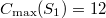 (see Figure 17.1), which can be easily proved to be the optimal value.
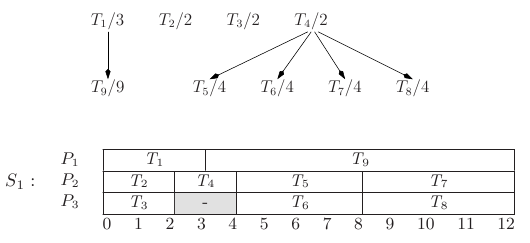
Example 17.5 Schedule the previous task system  for
for  equivalent processors with list
  . In this case for the resulting scheduling
  we get
 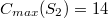 (see Figure 17.2).
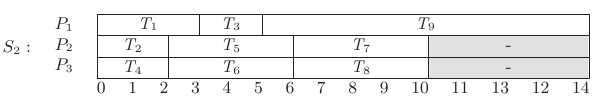
Example 17.6 Schedule the task system  with list
  for
for  processors. It results in
 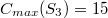 (see Figure 17.3).
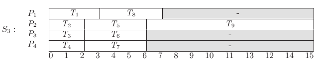
Example 17.7 Decrement the executing times by one in  . Schedule the resulting task system
  with list
  for
for  processors. The result is:
 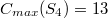 (see Figure 17.4).
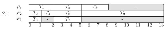
Example 17.8 Reduce the precedence restrictions: omit edges  and
and  from the graph. The result of scheduling
  of the resulting task system
  can be seen in Figure 17.5:
 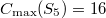 .
.
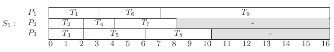
The following example shows that the increase of maximal finishing time in the worst case can be caused not only by a wrong choice of the list.
Example 17.9 Let task system  and its optimal scheduling
  be as showed by Figure 17.6. In this case
 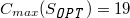 .
.
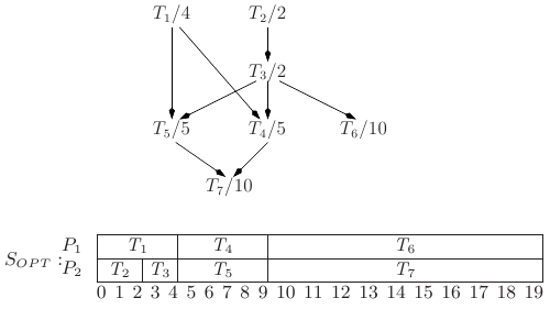
We can easily prove that if the executing times are decremented by one, then in the resulting task system  we cannot reach a better result than
  with any lists (see Figure 17.7).
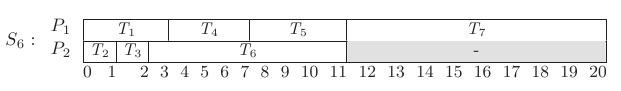
After these examples we give a relative limit reflecting the effects of the scheduling parameters. Suppose that for given task systems  and
and  we have
  ,
,  ,
,  . Task system
  is scheduled with the help of list
  , and
, and  with
with  — the former on
  , while the latter on
  equivalent processors. For the resulting schedulings
  and
and  let
let  and
and  .
.
Theorem 17.5 (scheduling limit) With the above conditions

Proof. Consider scheduling diagram  for the parameters with apostrophes (for
  ). Let the definition of two subsets—
  and
and  —of the interval
  be the following:
  ,
,  . Note that both sets are unions of disjoint, half-open (closed from the left and open from the right) intervals.
Let  be a task the execution of which ends in
  instant of time according to D1 (i. e.,
  ). In this case there are two possibilities: Starting point
  of task
  is either an inner point of
  , or not.
-
If
 is an inner point of
  , then according to the definition of
  there is a processor for which with
  it holds that it does not work in the interval
  . This can only occur if there is a task
  for which
  and
and  (case a).
 -
If
 is not an inner point of
  , then either
  (case b), or
  . If
. If  has got a smaller element than
  (case c), then let
  , else let
  (case d). If
  , then it follows from the construction of
  and
and  that there is a processor for which a task
  can be found the execution of which is still in progress in this time interval, and for which
  .
.
Summarising the two cases we can say that either there is a task  for which in the case of
  holds
holds  (case a or c), or for every number
 or
or  holds (case a or d).
Repeating this procedure we get a task chain  for which it holds that in the case of
  either
  or
or  . This proves that there are tasks for which

and in every instant of time  there is a processor which is working, and is executing one of the elements of the chain. It yields

where  denotes the empty periods, so the sum on the left hand side refers to all the empty periods in
  .
.
Based on (11.9) and  , therefore,

Since

and
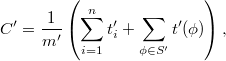
így (17.10), (17.11) and (17.12)
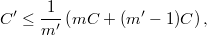
based on (17.10), (17.11) and (17.12) we get

implying 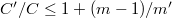 .
.
The following examples show us not only that the limit in the theory is the best possible, but also that we can get the given limit (at least asymptotically) by altering any of the parameters.
Example 17.10 In this example the list has changed, < is empty,  is arbitrary. Execution times are the following:
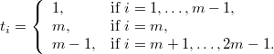
If this task system  is scheduled for
  processors with list
 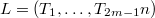 , then we get the optimal scheduling
  which can be seen in Figure 17.8.
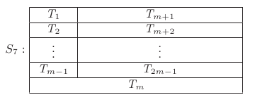
If we use the list  instead of list
  , then we get scheduling
  which can be seen in Figure 17.9.
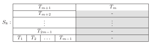
In this case  ,
,  , therefore
  ; which means that altering the list results in the theorem holding with equality, i.e., the expression on the right hand side of the
  sign cannot be decreased.
Example 17.11 In this example we decrease the execution times. We use list  . in both cases. Here as well as in the remaining part of the chapter
  denotes an arbitrarily small positive number. Original execution times are stored in vector
  , where
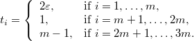
The new execution times are
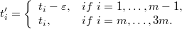
The precedence graph of task system  , and its modification
  are shown in Figure 17.10, while optimal scheduling
  and scheduling
  can be seen in Figure 17.11. Here
  and
and  C = Cmax, therefore, increasing
 goes to value
  (
( ). This means that altering the execution times we can approach the limit in the theorem arbitrarily closely.
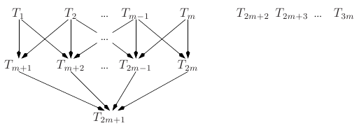
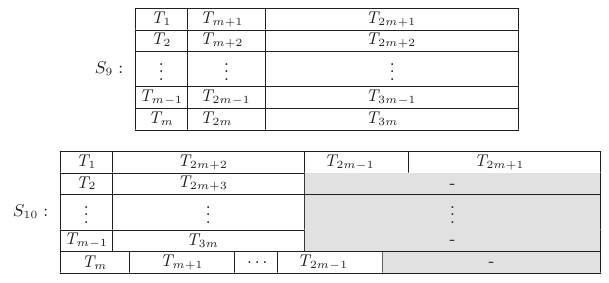
Example 17.12 In this example we reduce the precedence restrictions. The precedence graph of task system  is shown in Figure 17.12.
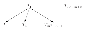
The execution times of the tasks are:  ,
,  , if
, if  , and
, and  . The optimal scheduling
  of
of  belonging to list
  can be seen in Figure 17.13.
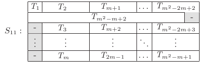
Omitting all the precedence restrictions from  we get the task system
  . Scheduling
  is shown in Figure 17.14.
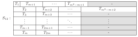
Example 17.13 This time the number of the processors will be increased from  to
to  . The graph of task system
  is shown by Figure 17.15, and the running times are
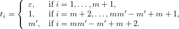
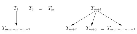
The optimal scheduling of the task system on  , and
, and  processors is shown by Figure 17.16 and Figure 17.17.
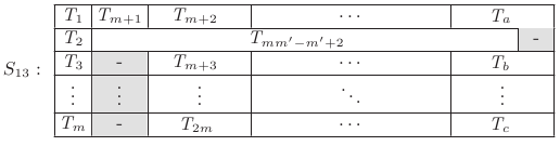
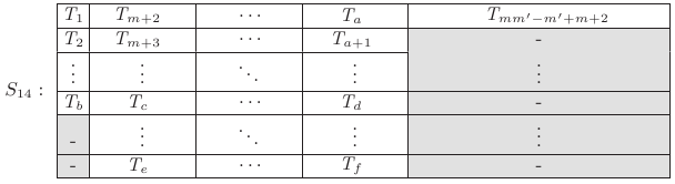
Comparing the  , and
, and  maximal finishing times we get the ratio
  and so again the required asymptotic value:
With the help of these examples we proved the following statement.
Theorem 17.6 (sharpness of the scheduling limit) The limit given for the relative speed (11.8) is asymptotically sharp for the changing of (any of the) parameters m, t, < and L.
We describe the parallel algorithm modelling the operating of computers with interleaved memory in a popular way. The sequence of dumplings is modelling the reference string, the giants the processors and the bites the commands executed simultaneously. Dwarfs  cook dumplings of
  different types. Every dwarf creates an infinite sequence of dumplings.
These sequences are usually given as random variables with possible values  . For the following analysis of the extreme cases deterministic sequences are used.
The dumplings eating giants  eat the dumplings. The units of the eating are the bits.
The appetite of the different giants is characterised by the parameter  . Giant
  is able to eat up most
  dumplings of the same sort at one bite.
Giant  eats the following way. He chooses for his first bite from the beginning from the beginning of the dumpling sequence of dwarf
  so many dumplings, as possible (at most
  of the same sort), and he adds to these dumplings so many ones from the beginning of the sequences of the dwarfs
  as possible.
After assembling the first bite the giant eats it, then he assembles and eats the second, third,  bites.
Example 17.14 To illustrate the model let us consider an example. We have two dwarfs ( and
and  ) and the giant
  . The dumpling sequences are

or in a shorter form

where the star (*) denotes a subsequence repeated infinitely many times.
For his first bite  chooses from the first sequence the first four dumlings 1212 (because the fifth dumpling is the third one of the sort 1) and no dumpling from the second sequence (because the beginning element is 2, and two dumplings of this sort is chosen already). The second bite contains the subsequence 1233 from the first sequence, and the dumplings 244 from the second one. The other bites are identical: 321321 from the first sequence and 44 from the second one. In a short form the bites are as follows:

(bites are separated by double lines).
For given dumpling sequences and a given giant  let
let  denote the number of dumplings in the
  -th bite. According to the eating-rules
  holds for every
  .
.
Considering the elements of the dumpling sequences as random variables with possible values  and given distribution we define the dumpling-eating speed
  (concerning the given sequences) of
  as the average number of dumplings in one bite for a long time, more precisely

where  denotes the expected value of the random variable
  .
.
One can see that the defined limit always exists.
Let us consider the case, when we have at least one dumpling sequence, at least one type of dumplings, and two different giants, that is let  . Let the sequences be deterministic.
Since for every bite-size  of
of  holds
holds  , the same bounds are right for every average value
  and for every expected value
  , too. From this it follows, that the limits
  and
and  defined in (17.16) also must lie between these bounds, that is

Choosing the maximal value of  and the minimal value of
  and vice versa we get the following trivial upper and lower bounds for the speed ratio
  :
:

Now we show that in many cases these trivial bounds cannot be improved (and so the dumpling eating speed of a small giant can be any times bigger than that of a big giant).
Theorem 17.7 If  , then there exist dumpling sequences, for which

further

Proof. To see the sharpness of the lower limit in the inequality (17.18) giving the natural limits let consider the following sequences:

Giant  eats these sequences in the following manner:

Here  ,
,  ,
,  ,
,  (for
(for  .
.
For the given sequences we have

 eats these sequences as follows:

Here


In this case we get (in a similar way, as we have got  )
)

and therefore

In order to derive the exact upper bound, we consider the following sequence:

 eats these sequences as follows:

From here we get

 'c eating is characterised by

where

Since  for
for  , therefore
  , and so
  .
.


We usually try to avoid anomalies.
For example at page replacing the sufficient condition of avoiding it is that the replacing algorithm should have the stack property: if the same reference string is run on computers with memory sizes of  and
and  , then after every reference it holds that the bigger memory contains all the pages that the smaller does. At the examined scheduling problem it is enough not to require the scheduling algorithm's using a list.
Exercises
17.3-1 Give parameters  and
and  so that the FIFO algorithm would cause at least three more page faults with a main memory of size
  than with that of size
  .
.
17.3-2 Give such parameters that using scheduling with list when increasing the number of processors the maximal stopping time increases at least to half as much again.
17.3-3 Give parameters with which the dumpling eating speed of a small giant is twice as big as that of a big giant.
In this section we will discuss a memory managing problem in which files with given sizes have to be placed onto discs with given sizes. The aim is to minimise the number of the discs used. The problem is the same as the bin-packing problem that can be found among the problems in Section Approximation algorithms in the book titled Introduction to Algorithms. Also scheduling theory uses this model in connection with minimising the number of processors. There is the number  of the files given, and array vector
  containing the sizes of the files to be stored, for the elements of which
  holds
holds  . The files have to be placed onto the discs taking into consideration that they cannot be divided and the capacity of the discs is a unit.
The given problem is NP-complete. Therefore, different approaching algorithms are used in practice. The input data of these algorithms are: the number  of files, a vector
  with the sizes of the files to be placed. And the output data are the number of discs needed (discnumber) and the level array
  of discs.
According to Linear Fit file  is placed to disc
  . The pseudocode of LF is the following.
LF(
)
1FOR
TO2
DO3
4
RETURN
Both the running time and the place requirement of this algorithm are  . If, however, reading the sizes and printing the levels are carried out in the loop in rows 2–3, then the space requirement can be decreased to
  .
.
Next Fit packs the files onto the disc next in line as long as possible. Its pseudocode is the following.
NF(
)
12
3
FOR
TO4
DOIF5
THEN6
ELSE7
8
RETURN
Both the running time and the place requirement of this algorithm are  . If, however, reading the sizes and taking the levels out are carried out in the loop in rows 3–6, then the space requirement can be decreased to
  , but the running time is still
  .
.
First Fit packs each files onto the first disc onto which it fits.
FF(
)
12
FOR
TO3
DO3
FOR
TO4
DO5
WHILE6
DO7
8
IF9
THEN10
RETURN
The space requirement of this algorithm is  , while its time requirement is
  . If, for example, every file size is 1, then the running time of the algorithm is
  .
.
Best Fit places each file onto the first disc on which the remaining capacity is the smallest.
BF(
)
12
FOR
TO3
DO4
FOR
TO5
DO6
7
FOR
TO8
DOIFand
9
THEN10
11
IF12
THEN13
ELSE14
15
RETURN
The space requirement of this algorithm is  , while its time requirement is
  .
.
Pairwise Fit creates a pair of the first and the last element of the array of sizes, and places the two files onto either one or two discs—according to the sum of the two sizes. In the pseudocode there are two auxiliary variables: bind is the index of the first element of the current pair, and eind is the index of the second element of the current pair.
PF(
)
12
3
4
WHILE5
DOIF6
THENIF7
THEN8
9
10
ELSE11
12
IF13
THEN14
15
16
17
RETURN
The space requirement of this algorithm is  , while its time requirement is
  . If, however, reading the sizes and taking the levels of the discs out are carried out online, then the space requirement will only be
  .
.
The following five algorithms consist of two parts: first they put the tasks into decreasing order according to their executing time, and then they schedule the ordered tasks. Next Fit Decreasing operates according to NF after ordering. Therefore, both its space and time requirement are made up of that of the applied ordering algorithm and NF.
First Fit Decreasing operates according to First Fit (FF) after ordering, therefore its space requirement is  and its time requirement is
  .
.
Best Fit Decreasing operates according to Best Fit (BF) after ordering, therefore its space requirement is  and its time requirement is
  .
.
Pairwise Fit Decreasing creates pairs of the first and the last tasks one after another, and schedules them possibly onto the same processor (if the sum of their executing time is not bigger than one). If it is not possible, then it schedules the given pair onto two processors.
Quick Fit Decreasing places the first file after ordering onto the next empty disc, and then adds the biggest possible files (found from the end of the ordered array of sizes) to this file as long as possible. The auxiliary variables used in the pseudocode are: bind is the index of the first file to be examined, and eind is the index of the last file to be examined.
QFD(
)
12
3
4
WHILE5
DO6
7
8
WHILEand
9
DO10
WHILEand
11
DO12
13
IF14
THENFOR
TO15
DO16
17
RETURN
The space requirement of this program is  , and its running time in worst case is
  , but in practice—in case of executing times of uniform distribution—it is
  .
.
This algorithm places each file—independently of each other—on each of the  discs, so it produces
  placing, from which it chooses an optimal one. Since this algorithm produces all the different packing (supposing that two placing are the same if they allocate the same files to all of the discs), it certainly finds one of the optimal placing.
This algorithm produces the permutations of all the files (the number of which is  ), and then it places the resulted lists using NF.
The algorithm being optimal can be proved as follows. Consider any file system and its optimal packing is  . Produce a permutation
  of the files based on
  so that we list the files placed onto
  respectively. If permutation
  is placed by NF algorithm, then we get either
  or another optimal placing (certain tasks might be placed onto processors with smaller indices).
This algorithm tries to decrease the time requirement of SP by placing 'large' files (the size of which is bigger than 0.5) on separate discs, and tries to place only the others (the 'small' ones) onto all the  discs. Therefore, it produces only
  placing instead of
  , where
  is the number of small files.
This algorithm also takes into consideration that two small files always fit onto a disc—besides the fact that two large ones do not fit. Therefore, denoting the number of large files by  and that of the small ones by
  it needs at most
  discs. So first we schedule the large discs to separate discs, and then the small ones to each of the discs of the number mentioned above. If, for instance,
  , then according to this we only have to produce
  .
.
With certain conditions it holds that list  can be split into lists
  and
and  so that
  (in these cases the formula holds with equality). Its advantage is that usually shorter lists can be packed optimally in a shorter time than the original list. For example, let us assume that
  . Let
. Let  and
and  . In this case
  and
and  . To prove this, consider the two discs onto which the elements of list
  have been packed by an optimal algorithm. Since next to them there can be files whose sum is at most
  and
and  , their executing time can sum up to at most
  , i.e., 1. Examining the lists on both ends at the same time we can sort out the pairs of files the sum of whose running time is 1 in
  . After that we order the list
  . Let the ordered list be s. If, for example
  , then the first file will be packed onto a different disc by every placing, so
  and
and  is a good choice. If for the ordered list
  and
and  hold, then let
  be the largest element of the list that can be added to
  without exceeding one. In this case with choices
  and
and  list
list  is two elements shorter than list
  . With the help of the last two operations lists can often be shortened considerably (in favourable case they can be shortened to such an extent that we can easily get the optimal number of processors for both lists). Naturally, the list remained after shortening has to be processed—for example with one of the previous algorithms.
Algorithms based on upper and lower estimations operate as follows. Using one of the approaching algorithms they produce an upper estimation A  of OPT(
 ), and then they give a lower estimation for the value of OPT(
 as well. For this—among others—the properties of packing are suitable, according to which two large files cannot be placed onto the same disc, and the sum of the size cannot be more than 1 on any of the discs. Therefore, both the number of the large files and the sum of the size of the files, and so also their maximum MAX(
 ) is suitable as a lower estimation. If A(
 MAX(
MAX( ), then algorithm A produced an optimal scheduling. Otherwise it can be continued with one of the time-consuming optimum searching algorithms.
If there are several algorithms known for a scheduling (or other) problem, then a simple way of comparing the algorithms is to examine whether the values of the parameters involved can be given so that the chosen output value is more favourable in the case of one algorithm than in the case of the other one.
In the case of the above discussed placing algorithm the number of processors discs allocated to size array t by algorithm A and B is denoted by A(t and B(t, and we examine whether there are arrays  and
and  for which A(
 ) < B(
 ) and A(
 ) > B(
 ) hold. We answer this question in the case of the above defined ten approaching algorithms and for the optimal one. It follows from the definition of the optimal algorithms that for each t and each algorithm A holds OPT
  A
A  . In the following the elements of the arrays in the examples will be twentieth.
Consider the following seven lists:  ,
,
 ,
,
 ,
,
 ,
,
 ,
,
 ,
,
 .
.
The packing results of these lists are summarised in Figure 17.18.
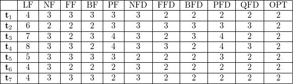
As shown in Figure 17.18, LF needs four discs for the first list, while the others need fewer than that. In addition, the row of list  shows that FFD, BFD, PFD, QFD and OPT need fewer discs than NF, FF, BF, PF and NFD. Of course, there are no lists for which any of the algorithms would use fewer discs than OPT. It is also obvious that there are no lists for which LF would use fewer discs than any of the other ten algorithms.
These facts are shown in Figure 17.19. In the figure symbols X in the main diagonal indicate that the algorithms are not compared to themselves. Dashes in the first column indicate that for the algorithm belonging to the given row there is no list which would be processed using more disc by this algorithm than by the algorithm belonging to the given column, i.e., LF. Dashes in the last column show that there is no list for which the optimal algorithm would use more discs than any of the examined algorithms. Finally, 1's indicate that for list  the algorithm belonging to the row of the given cell in the figure needs more discs than the algorithm belonging to the column of the given cell.
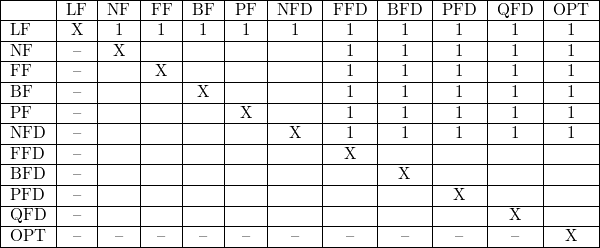
If we keep analysing the numbers of discs in Figure 17.19, we can make up this figure to Figure 17.20.
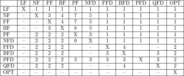
Since the first row and the first column of the table is filled, we do not deal more with algorithm LF.
For list  NF, FF, BF and OPT use two discs, while the other 6 algorithms use three ones. Therefore we write 2's in the points of intersection of the columns of the 'winners' and the rows of the 'losers' (but we do not rewrite the 1's given in the points of intersection of PF and OPT, and NFD and OPT, so we write 2's in
  cells. Since both the row and the column of OPT have been filled in, it is not dealt with any more in this section. The third list is disadvantageous for PF and PFD, therefore we write 3's in the empty cells in their rows. This list shows an example also for the fact that NF can be worse than FF, BF can be worse than FF, and BFD than FFD and QFD.
The fourth list can be processed only by BF and BFD optimally, i.e., using two discs. Therefore we can write 4's in the empty cells in the columns of these two algorithms. For the fifth list NFD, FFD, BFD and QFD use only two, while NF, FF, BF, PF and PDF use three discs. So we can fill the suitable cells with 5's. The 'losers' of list  are NF and NFD—therefore, we write 6's in the empty cells in their rows. PF performs better when processing list
  than FF. The following theorem helps us filling in the rest of the cells.
 , then
Proof. We perform an induction according to the length of the list. Let  and
and  . Let NF
  N
N  and FF
  F
F  , and let
  be the level of the last disc according to NF, which means the sum of the lengths of the files placed onto the non empty disc with the higher index, when NF has just processed
  . Similarly, let
  be the level of the last disc according to FF. We are going to prove the following invariant property for each
  : either
  , or
, or  and
and  . If
. If  , then
  and
and  , i.e., the second part of the invariant property holds. Suppose that the property holds for the value
  . If the first part of the invariant property holds before packing
  , then either inequality
  stays true, or the numbers of discs are equal, and
  holds. If the numbers of discs were equal before packing of
  , then after placing it either the number of discs of FF is smaller, or the numbers of discs are equal and the level of the last disc of FF is at most as big as that of NF.
A similar statement can be proved for the pairs of algorithms NF-BF, NFD-FFD and NFD-BFD. Using an induction we could prove that FFD and QFD need the same number of discs for every list. The previous statements are summarised in Figure 11.20.
The relative efficiency of two algorithms (A and B) is often described by the ratio of the values of the chosen efficiency measures, this time the relative number of processors  . Several different characteristics can be defined using this ratio. These can be divided into two groups: in the first group there are the quantities describing the worst case, while in the other group there are those describing the usual case. Only the worst case is going to be discussed here (the discussion of the usual case is generally much more difficult). Let
  denote the real list of
  elements and
  the set of all the real lists, i.e.,

Let  be the set of algorithms, determining the number of discs, that is of algorithms, connecting a nonnegative real number to each list
  , so implementing the mapping
  ).
).
Let  be the set of the optimal algorithms, that is of algorithms ordering the optimal number of discs to each list, and OPT an element of this set (i.e., an algorithm that gives the number of discs sufficient and necessary to place the files belonging to the list for each list
  ).
).
Let  be the set of the approximation algorithms, that is of algorithms
  for which
  for each list
  , and there is a list
  , for which
  .
.
Let  be the set of estimation algorithms, that is of algorithms
  for which
  for each list
  , and there is a list
  , for which
  . Let
. Let  denote the set of real lists for which
  , i.e.,
 . In the following we discuss only algorithms contained in
  . We define
  error function,
  error (absolute error) and
  asymptotic error of algorithms A and B
  as follows:
These quantities are interesting especially if  . In this case, to be as simple as possible, we omit B from the denotations, and speak about the error function, error and asymptotic error of algorithms
  , and
, and  . The characteristic values of NF file placing algorithm are known.
 , then
Furthermore, if  , then there are lists
  and
and  for which

and

From this statement follows the error function, absolute error and asymptotic error of NF placing algorithm.
 then
then
and

The following statement refers to the worst case of the FF and BF file packing algorithms.
 , then
Furthermore, if  , then there are lists
  and
and  for which

and

For the algorithm FF holds the following stronger upper bound too.
 , then
From this statement follows the asymptotic error of FF and BF, and the good estimation of their error function.
 , then
and

further

If  is divisible by 10, then the upper and lower limits in inequality (17.40) are equal, thus in this case
  .
.
Exercises
17.4-1 Prove that the absolute error of the FF and BF algorithms is at least 1.7 by an example.
17.4-2 Implement the basic idea of the FF and BF algorithms so that the running time would be  .
.
17.4-3 Complete Figure 11.20.
PROBLEMS |
17-1 Smooth process selection for an empty partition
Modify the Long-Waiting-or-Not-Fit-Smaller algorithm in a way that instead of giving priority to processes with  above the
  , selects the process with the highest
  among the processes fitting into the partition. Prove the correctness of the algorithm and give an upper bound for the waiting time of a process.
17-2 Partition search algorithms with restricted scope
Modify the Best-Fit, Limited-Best-Fit, Worst-Fit, Limited-Worst-Fit algorithms to only search for their optimal partitions among the next  suitable one following the last split partition, where
  is a fixed positive number. Which algorithms do we get in the
  and
and  cases. Simulate both the original and the new algorithms, and compare their performance regarding execution time, average number of waiting processes and memory fragmentation.
17-3 Avoiding page replacement anomaly
Class the discussed page replacement algorithms based on whether they ensure to avoid the anomaly or not.
17-4 Optimal page replacement algorithm
Prove that for each demanding page replacement algorithm  , memory size
  and reference string
  holds
holds
17-5 Anomaly
Plan (and implement) an algorithm with which it can occur that a given problem takes longer to solve on  processors than on
  ones.
ones.
17-6 Error of file placing algorithms
Give upper and lower limits for the error of the BF, BFD, FF and FFD algorithms.
CHAPTER NOTES |
The basic algorithms for dynamic and fixed partitioning and page replacement are discussed according to textbooks by Silberschatz, Galvin and Gagne [303], and Tanenbaum and Woodhull [316].
Defining page replacement algorithms by a Mealy-automat is based on the summarising article by Denning [87], and textbooks by Ferenc Gécseg and István Peák [131], Hopcroft, Motwani and Ullman [166].
Optimizing the MIN algorithm was proved by Mihnovskiy and Shor in 1965 [244], after that by Mattson, Gecsei, Slutz and Traiger in 1970 [236].
The anomaly experienced in practice when using FIFO page replacement algorithm was first described by László Bélády [43] in 1966, after that he proved in a constructive way that the degree of the anomaly can approach two arbitrarily closely in his study he wrote together with Shedler. The conjecture that it cannot actually reach two can be found in the same article (written in 1969).
Péter Formai and Antal Iványi [115] showed that the ratio of the numbers of page replacements needed on a big and on a smaller computer can be arbitrarily large in 2002.
Examples for scheduling anomalies can be found in the books by Coffman [71], Iványi and Smelyanskiy [179] and Roosta [290], and in the article by Lai and Sahni [209].
Analysis of the interleaved memory derives from the article [175].
The bound  can be found in D. S. Johnson's PhD dissertation [184], the precise Theorem 17.9. comes from [177]. The upper limit for FF and BF is a result by Johnson, Demers, Ullman, Garey and Graham [185], while the proof of the accuracy of the limit is that by [177], [178]. The source of the upper limit for FFD and BFD is [185], and that of the limit for NFD is [27]. The proof of the NP-completeness of the file packing problem—leading it back to the problem of partial sum—can be found in the chapter on approximation algorithms in Introduction to Algorithms [73].
Table of Contents
The relational datamodel was introduced by Codd in 1970. It is the most widely used datamodel—extended with the possibilities of the World Wide Web—, because of its simplicity and flexibility. The main idea of the relational model is that data is organised in relational tables, where rows correspond to individual records and columns to attributes. A relational schema consists of one or more relations and their attribute sets. In the present chapter only schemata consisting of one relation are considered for the sake of simplicity. In contrast to the mathematical concept of relations, in the relational schema the order of the attributes is not important, always sets of attributes are considered instead of lists. Every attribute has an associated domain that is a set of elementary values that the attribute can take values from. As an example, consider the following schema.
| Employee(Name,Mother's name,Social Security Number,Post,Salary) |
The domain of attributes Name and Mother's name is the set of finite character strings (more precisely its subset containing all possible names). The domain of Social Security Number is the set of integers satisfying certain formal and parity check requirements. The attribute Post can take values from the set {Director,Section chief,System integrator,Programmer,Receptionist,Janitor,Handyman}. An instance of a schema  is a relation
  if its columns correspond to the attributes of
  and its rows contain values from the domains of attributes at the attributes' positions. A typical row of a relation of the Employee schema could be
| (John Brown,Camille Parker,184-83-2010,Programmer,$172,000) |
There can be dependencies between different data of a relation. For example, in an instance of the Employee schema the value of Social Security Number determines all other values of a row. Similarly, the pair (Name,Mother's name) is a unique identifier. Naturally, it may occur that some set of attributes do not determine all attributes of a record uniquely, just some of its subsets.
A relational schema has several integrity constraints attached. The most important kind of these is functional dependency. Let  and
and  be two sets of attributes.
  functionally depends on
  ,
,  in notation, means that whenever two records are identical in the attributes belonging to
  , then they must agree in the attribute belonging to
  , as well. Throughout this chapter the attribute set
  is denoted by
  for the sake of convenience.
Example 18.1 Functional dependencies Consider the schema
| R(Professor,Subject,Room,Student,Grade,Time). |
The meaning of an individual record is that a given student got a given grade of a given subject that was taught by a given professor at a given time slot. The following functional dependencies are satisfied.
-
Su
 P: One subject is taught by one professor.
 -
PT
 R: A professor teaches in one room at a time.
 -
StT
 R: A student attends a lecture in one room at a time.
 -
StT
 Su: A student attends a lecture of one subject at a time.
 -
SuSt
 G: A student receives a unique final grade of a subject.
In Example 18.1 the attribute set StT uniquely determines the values of all other attributes, furthermore it is minimal such set with respect to containment. This kind attribute sets are called keys. If all attributes are functionally dependent on a set of attributes  , then
  is called a superkey. It is clear that every superkey contains a key and that any set of attributes containing a superkey is also a superkey.
Some functional dependencies valid for a given relational schema are known already in the design phase, others are consequences of these. The StT  P dependency is implied by the StT
  Su and Su
  P dependencies in Example 18.1. Indeed, if two records agree on attributes St and T, then they must have the same value in attribute Su. Agreeing in Su and Su
  P implies that the two records agree in P, as well, thus StT
  P holds.
Definition 18.1 Let  be a relational schema,
  be a set of functional dependencies over
  . The functional dependency
  is logically implied by
  , in notation
  , if each instance of
  that satisfies all dependencies of
  also satisfies
  . The closure of a set
  of functional dependencies is the set
  given by

In order to determine keys, or to understand logical implication between functional dependencies, it is necessary to know the closure  of a set
  of functional dependencies, or for a given
  dependency the question whether it belongs to
  must be decidable. For this, inference rules are needed that tell that from a set of functional dependencies what others follow. The Armstrong-axioms form a system of sound and complete inference rules. A system of rules is sound if only valid functional dependencies can be derived using it. It is complete, if every dependency
  that is logically implied by the set
  is derivable from
  using the inference rules.
Armstrong-axioms
-
(A1) Reflexivity
 implies
  .
. -
(A2) Augmentation If
 , then for arbitrary
  ,
,  holds.
 -
(A3) Transitivity If
 and
and  hold, then
  holds, as well.
Example 18.2 Derivation by the Armstrong-axioms. Let  and
and  , then
  is a key:
-
 is given.
 -
 1. is augmented by (A2) with
  .
. -
 is given.
 -
 3. is augmented by (A2) with
  .
. -
 transitivity (A3) is applied to 2. and 4.
Thus it is shown that  is superkey. That it is really a key, follows from algorithm
 Closure(
).
There are other valid inference rules besides (A1)–(A3). The next lemma lists some, the proof is left to the Reader (Exercise 18.1-5).
-
Union rule
 .
. -
Pseudo transitivity
 .
. -
Decomposition If
 holds and
  , then
  holds, as well.
The soundness of system (A1)–(A3) can be proven by easy induction on the length of the derivation. The completeness will follow from the proof of correctness of algorithm Closure(
) by the following lemma. Let  denote the closure of the set of attributes
  with respect to the family of functional dependencies
  , that is
  .
.
Lemma 18.3 The functional dependency  follows from the family of functional dependencies
  by the Armstrong-axioms iff
  .
.
Proof. Let  where
where  's are attributes, and assume that
  .
.  follows by the Armstrong-axioms for all
  by the definition of
  . Applying the union rule of Lemma 18.2
  follows. On the other hand, assume that
  can be derived by the Armstrong-axioms. By the decomposition rule of Lemma 18.2
  follows by (A1)–(A3) for all
  . Thus,
  .
.
Calculation of closures is important in testing equivalence or logical implication between systems of functional dependencies. The first idea could be that for a given family  of functional dependencies in order to decide whether
  , it is enough to calculate
  and check whether
  holds. However, the size of
  could be exponential in the size of input. Consider the family
  of functional dependencies given by

 consists of all functional dependencies of the form
  , where
  , thus
  . Nevertheless, the closure
  of an attribute set
  with respect to
  can be determined in linear time of the total length of functional dependencies in
  . The following is an algorithm that calculates the closure
  of an attribute set
  with respect to
  . The input consists of the schema
  , that is a finite set of attributes, a set
  of functional dependencies defined over
  , and an attribute set
  .
.
Closure(
)
12
3

Functional dependencies not used yet. 4
REPEAT56
FORallin
7
DOIF8
THEN9
10
11
UNTIL
It is easy to see that the attributes that are put into any of the  's by
's by Closure(
) really belong to  . The harder part of the correctness proof of this algorithm is to show that each attribute belonging to
  will be put into some of the
  's.
's.
Theorem 18.4 Closure(
) correctly calculates  .
.
Proof. First we prove by induction that if an attribute  is put into an
  during
 Closure(
), then  really belongs to
  .
.
Base case:  . I this case
  and by reflexivity (A1)
  .
.
Induction step: Let  and assume that
  .
.  is put into
  , because there is a functional dependency
  in
in  , where
  and
and  . By induction,
  holds, which implies using Lemma 18.3 that
  holds, as well. By transitivity (A3)
  and
and  implies
  . By reflexivity (A1) and
  ,
,  holds. Applying transitivity again,
  is obtained, that is
  .
.
On the other hand, we show that if  , then
  is contained in the result of
 Closure(
). Suppose in contrary that  , but
, but  , where
  is the result of
 Closure(
). By the stop condition in line 9 this means  . An instance
  of the schema
  is constructed that satisfies every functional dependency of
  , but
, but  does not hold in
  if
if  . Let
. Let  be the following two-rowed relation:
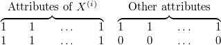
Let us suppose that the above  violates a
  functional dependency of
  , that is
  , but
, but  is not a subset of
  . However, in this case
 Closure(
) could not have stopped yet, since  .
.
 implies using Lemma 18.3 that
  follows from
  by the Armstrong-axioms. (A1)–(A3) is a sound system of inference rules, hence in every instance that satisfies
  ,
,  must hold. However, the only way this could happen in instance
  is if
is if  .
.
Let us observe that the relation instance  given in the proof above provides the completeness proof for the Armstrong-axioms, as well. Indeed, the closure
  calculated by
 Closure(
) is the set of those attributes for which  follows from
  by the Armstrong-axioms. Meanwhile, for every other attribute
  , there exist two rows of
  that agree on
  , but differ in
  , that is
  does not hold.
The running tome of Closure(
) is  , where
  is the length of he input. Indeed, in the
 rEPEAT – uNTIL loop of lines 4–11 every not yet used dependency is checked, and the body of the loop is executed at most  times, since it is started again only if
  , that is a new attribute is added to the closure of
  . However, the running time can be reduced to linear with appropriate bookkeeping.
-
For every yet unused
 dependency of
  it is kept track of how many attributes of
  are not yet included in the closure (
 ).
). -
For every attribute
 those yet unused dependencies are kept in a doubly linked list
  whose left side contains
  .
. -
Those not yet used dependencies
 are kept in a linked list
  , whose left side
  's every attribute is contained in the closure already, that is for which
  .
.
It is assumed that the family of functional dependencies  is given as a set of attribute pairs
  , representing
  . The
. The Linear-Closure(
) algorithm is a modification of Closure(
) using the above bookkeeping, whose running time is linear.  is the schema,
  is the given family of functional dependencies, and we are to determine the closure of attribute set
  .
.
Algorithm Linear-Closure(
) consists of two parts. In the initialisation phase (lines 1–13) the lists are initialised. The loops of lines 2–5 and 6–8, respectively, take  time. The loop in lines 9–11 means
  steps. If the length of the input is denoted by
  , then this is
  steps altogether.
During the execution of lines 14–23, every functional dependency  is examined at most once, when it is taken off from list
  . Thus, lines 15–16 and 23 take at most
  steps. The running time of the loops in line 17–22 can be estimated by observing that the sum
  is decreased by one in each execution, hence it takes
  steps, where
  is the
  value obtained in the initialisation phase. However,
  , thus lines 14–23 also take
  time in total.
Linear-Closure(
)
1Initialisation phase. 2
FORall3
DOFORall4
DOaddto list
5
6
FORall7
DOFORallof list
8
DO9
FORall10
DOIF11
THENaddto list
12
13
End of initialisation phase. 14
WHILEis nonempty 15
DO16 delete
from list
17
FORall18
DOFORallof list
19
DO20
IF21
THENaddto list
22 delete
from list
23
24
RETURN

Algorithm Linear-Closure(
) can be used to test equivalence of systems of dependencies. Let  and
and  be two families of functional dependencies.
  and
and  are said to be equivalent, if exactly the same functional dependencies follow from both, that is
  . It is clear that it is enough to check for all functional dependencies
  in
in  whether it belongs to
  , and vice versa, for all
  in
in  , whether it is in
  . Indeed, if some of these is not satisfied, say
  is not in
  , then surely
  . On the other hand, if all
  are in
  , then a proof of a functional dependency
  from
from  can be obtained from dependencies in
  in such a way that to the derivation of the dependencies
  of
of  from
from  , the derivation of
  from
from  is concatenated. In order to decide that a dependency
  from
from  is in
is in  , it is enough to construct the closure
  of attribute set
  with respect to
  using
using Linear-Closure(
), then check whether  holds. The following special functional dependency system equivalent with
  is useful.
Definition 18.5 The system of functional dependencies  is a minimal cover of the family of functional dependencies
  iff
iff  is equivalent with
  , and
, and
-
functional dependencies of
 are in the form
  , where
  is an attribute and
  ,
, -
no functional dependency can be dropped from
 , i.e.,
  ,
, -
the left sides of dependencies in
 are minimal, that is
  ,
,  .
.
Every set of functional dependencies have a minimal cover, namely algorithm Minimal-Cover(
) constructs one.
Minimal-Cover(
)
12
FORall3
DOFORall4
DO5
Each right hand side consists of a single attribute. 6
FORall7
DOWHILEthere exists8
9
Each left hand side is minimal. 10
FORall11
DOIF12
THEN13
No redundant dependency exists.
After executing the loop of lines 2–4, the right hand side of each dependency in  consists of a single attribute. The equality
  follows from the union rule of Lemma 18.2 and the reflexivity axiom. Lines 6–8 minimise the left hand sides. In line 11 it is checked whether a given functional dependency of
  can be removed without changing the closure.
  is the closure of attribute set
  with respect to the family of functional dependencies
  .
.
Claim 18.6 Minimal-Cover(
) calculates a minimal cover of  .
.
Proof. It is enough to show that during execution of the loop in lines 10–12, no functional dependency  is generated whose left hand side could be decreased. Indeed, if a
  dependency would exist, such that for some
 held, then
  would also hold, where
  is the set of dependencies considered when
  is checked in lines 6–8.
  , which implies
  (see Exercise 18.1-1). Thus,
  should have been decreased already during execution of the loop in lines 6–8.
In database design it is important to identify those attribute sets that uniquely determine the data in individual records.
Definition 18.7 Let  be a relational schema. The set of attributes
  is called a superkey, if
  . A superkey
  is called a key, if it is minimal with respect to containment, that is no proper subset
  is key.
The question is how the keys can be determined from  ? What makes this problem hard is that the number of keys could be super exponential function of the size of
  . In particular, Yu and Johnson constructed such relational schema, where
  , but the number of keys is
  . Békéssy and Demetrovics gave a beautiful and simple proof of the fact that starting from
  functional dependencies, at most
  key can be obtained. (This was independently proved by Osborne and Tompa.)
The proof of Békéssy and Demetrovics is based on the operation  they introduced, which is defined for functional dependencies.
Definition 18.8 Let  and
and  be two functional dependencies. The binary operation
  is defined by

Some properties of operation  is listed, the proof is left to the Reader (Exercise 18.1-3). Operation
  is associative, furthermore it is idempotent in the sense that if
  and
and  for some
  , then
  .
.
Claim 18.9 (Békéssy and Demetrovics) Let  be a relational schema and let
  be a listing of the functional dependencies. If
  is a key, then
  , where
  is an ordered subset of the index set
  , and
, and  is a trivial dependency in the form
  .
.
Proposition 18.9 bounds in some sense the possible sets of attributes in the search for keys. The next proposition gives lower and upper bounds for the keys.
Claim 18.10 Let  be a relational schema and let
  . Let us assume without loss of generality that
  . Let
. Let  and
and  . If
. If  is a key in the schema
  , then

The proof is not too hard, it is left as an exercise for the Reader (Exercise 18.1-4). The algorithm List-keys(
) that lists the keys of the schema  is based on the bounds of Proposition 18.10. The running time can be bounded by
  , but one cannot expect any better, since to list the output needs that much time in worst case.
List-Keys(
)
1Let
and
be as defined in Proposition 18.10 2
IF3
THENRETURN4

is the only key. 5
IF6
THENRETURN7

is the only key. 8
9
FORall permutationsof the attributes of
10
DO11
FOR
TO12
DO13
IF14
THEN15
16
RETURN
Exercises
18.1-1 Let  be a relational schema and let
  and
and  be families of functional dependencies over
  . Show that
a.  .
.
b.  .
.
c. If  , then
  .
.
Formulate and prove similar properties of the closure  – with respect to
  – of an attribute set
  .
.
18.1-2 Derive the functional dependency  from the set of dependencies
  using Armstrong-axioms (A1)–(A3).
18.1-3 Show that operation  is associative, furthermore if for functional dependencies
  we have
  and
and  for some
  , then
  .
.
18.1-4 Prove Proposition 18.10.
18.1-5 Prove the union, pseudo transitivity and decomposition rules of Lemma 18.2.
A decomposition of a relational schema  is a collection
  of subsets of
  such that

The  's need not be disjoint, in fact in most application they must not be. One important motivation of decompositions is to avoid anomalies.
Example 18.3 Anomalies Consider the following schema
| SUPPLIER-INFO(SNAME,ADDRESS,ITEM,PRICE) |
This schema encompasses the following problems:
-
Redundancy. The address of a supplier is recorded with every item it supplies.
-
Possible inconsistency (update anomaly). As a consequence of redundancy, the address of a supplier might be updated in some records and might not be in some others, hence the supplier would not have a unique address, even though it is expected to have.
-
Insertion anomaly. The address of a supplier cannot be recorded if it does not supply anything at the moment. One could try to use
NULLvalues in attributes ITEM and PRICE, but would it be remembered that it must be deleted, when a supplied item is entered for that supplier? More serious problem that SNAME and ITEM together form a key of the schema, and theNULLvalues could make it impossible to search by an index based on that key. -
Deletion anomaly. This is the opposite of the above. If all items supplied by a supplier are deleted, then as a side effect the address of the supplier is also lost.
All problems mentioned above are eliminated if schema SUPPLIER-INFO is replaced by two sub-schemata:
| SUPPLIER(SNAME,ADDRESS), |
| SUPPLIES(SNAME,ITEM,PRICE). |
In this case each suppliers address is recorded only once, and it is not necessary that the supplier supplies a item in order its address to be recorded. For the sake of convenience the attributes are denoted by single characters  (SNAME),
  (ADDRESS),
  (ITEM),
  (PRICE).
Question is that is it correct to replace the schema  by
by  and
and  ? Let
? Let  be and instance of schema
  . It is natural to require that if
  and
and  is used, then the relations belonging to them are obtained projecting
  to
to  and
and  , respectively, that is
  and
and  .
.  and
and  contains the same information as
  , if
, if  can be reconstructed using only
  and
and  . The calculation of
  from
from  and
and  can bone by the natural join operator.
Definition 18.11 The natural join of relations  of schemata
  (
( ) is the relation
  belonging to the schema
  , which consists of all rows
  that for all
  there exists a row
  of relation
  such that
  . In notation
  .
.
Example 18.4 Let  ,
,  ,
,  and
and  . The natural join of
  and
and  belongs to the schema
  , and it is the relation
  .
.
If  is the natural join of
  and
and  , that is
  , then
  és
és  by Lemma 18.12. If
  , then the original relation could not be reconstructed knowing only
  and
and  .
.
Let  be a decomposition of schema
  , furthermore let
  be a family of functional dependencies over
  . The decomposition
  is said to have lossless join property (with respect to
  ), if every instance
  of
of  that satisfies
  also satisfies

That is, relation  is the natural join of its projections to attribute sets
  ,
,  . For a decomposition
  , let
, let  denote the the mapping which assigns to relation
  the relation
  . Thus, the lossless join property with respect to a family of functional dependencies means that
  for all instances
  that satisfy
  .
.
Lemma 18.12 Let  be a decomposition of schema
  , and let
  be an arbitrary instance of
  . Furthermore, let
  . Then
-
 .
. -
If
 , then
  .
. -
 .
.
The proof is left to the Reader (Exercise 18.2-7).
It is relatively not hard to check that a decomposition  of schema
  has the lossless join property. The essence of algorithm
 Join-Test(
) is the following.
A  array
array  is constructed, whose column
  corresponds to attribute
  , while row
  corresponds to schema
  .
.  if
if  , otherwise
  .
.
The following step is repeated until there is no more possible change in the array. Consider a functional dependency  from
from  . If a pair of rows
  and
and  agree in all attributes of
  , then their values in attributes of
  are made equal. More precisely, if one of the values in an attribute of
  is
is  , then the other one is set to
  , as well, otherwise it is arbitrary which of the two values is set to be equal to the other one. If a symbol is changed, then each of its occurrences in that column must be changed accordingly. If at the end of this process there is an all
  row in
  , then the decomposition has the lossless join property, otherwise, it is lossy.
Join-Test(
)
1Initialisation phase. 2
FOR
TO3
DOFOR
TO4
DOIF5
THEN6
ELSE7
End of initialisation phase. 8
9
REPEAT1011
FORall12
DOFOR
TO13
DOFOR
TO14
DOIFfor allin

15
THENEquate()16UNTIL17
IFthere exist an all 0 row in18
THENRETURN“Lossless join” 19ELSERETURN“Lossy join”

Procedure Equate(
) makes the appropriate symbols equal.
Equate(
)
1FOR2
DOIF3
THEN4FORTO5
DOIF6
THEN7
ELSE8FOR
TO9
DOIF10
THEN

Example 18.5 Checking lossless join property Let  ,
,  ,
,  ,
,  ,
,  ,
,  , furthermore let the functional dependencies be
  . The initial array is shown on Figure 18.1(a). Using
  values 1,2,5 in column
  can be equated to 1. Then applying
  value 3 of column
  again can be changed to 1. The result is shown on Figure 18.1(b). Now
  can be used to change values 2,3,5 of column
  to 0. Then applying
  (the only nonzero) value 1 of column
  can be set to 0. Finally,
  makes it possible to change values 3 and 4 in column
  to be changed to 0. The final result is shown on Figure 18.1(c). The third row consists of only zeroes, thus the decomposition has the lossless join property.
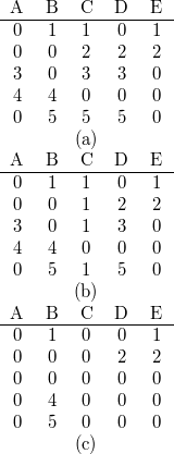
It is clear that the running time of algorithm Join-test(
) is polynomial in the length of the input. The important thing is that it uses only the schema, not the instance  belonging to the schema. Since the size of an instance is larger than the size of the schema by many orders of magnitude, the running time of an algorithm using the schema only is negligible with respect to the time required by an algorithm processing the data stored.
Theorem 18.13 Procedure Join-test(
) correctly determines whether a given decomposition has the lossless join property.
Proof. Let us assume first that the resulting array  contains no all zero row.
  itself can be considered as a relational instance over the schema
  . This relation satisfies all functional dependencies from
  , because the algorithm finished since there was no more change in the table during checking the functional dependencies. It is true for the starting table that its projections to every
  's contain an all zero row, and this property does not change during the running of the algorithm, since a 0 is never changed to another symbol. It follows, that the natural join
  contains the all zero row, that is
  . Thus the decomposition is lossy. The proof of the other direction is only sketched.
Logic, domain calculus is used. The necessary definitions can be found in the books of Abiteboul, Hull and Vianu, or Ullman, respectively. Imagine that variable  is written in place of zeroes, and
  is written in place of
  's in column
  , and
, and Join-test(
) is run in this setting. The resulting table contains row  , which corresponds to the all zero row. Every table can be viewed as a shorthand notation for the following domain calculus expression

where  is the
  th row of
  . If
. If  is the starting table, then formula (18.1) defines
  exactly. As a justification note that for a relation
  ,
,  contains the row
  iff
iff  contains for all
  a row whose
  th coordinate is
  if
if  is an attribute of
  , and arbitrary values represented by variables
  in the other attributes.
Consider an arbitrary relation  belonging to schema
  that satisfies the dependencies of
  . The modifications (equating symbols) of the table done by
 Join-test(
) do not change the set of rows obtained from  by (18.1), if the modifications are done in the formula, as well. Intuitively it can be seen from the fact that only such symbols are equated in (18.1), that can only take equal values in a relation satisfying functional dependencies of
  . The exact proof is omitted, since it is quiet tedious.
Since in the result table of Join-test(
) the all  's row occurs, the domain calculus formula that belongs to this table is of the following form:

It is obvious that if (18.2) is applied to relation  belonging to schema
  , then the result will be a subset of
  . However, if
  satisfies the dependencies of
  , then (18.2) calculates
  . According to Lemma 18.12,
  holds, thus if
  satisfies
  , then (18.2) gives back
  exactly, so
  , that is the decomposition has the lossless join property.
Procedure Join-test(
) can be used independently of the number of parts occurring in the decomposition. The price of this generality is paid in the running time requirement. However, if  is to be decomposed only into two parts, then
 Closure(
) or Linear-Closure(
) can be used to obtain the same result faster, according to the next theorem.
Theorem 18.14 Let  be a decomposition of
  , furthermore let
  be a set of functional dependencies. Decomposition
  has the lossless join property with respect to
  iff
iff

These dependencies need not be in  , it is enough if they are in
  .
.
Proof. The starting table in procedure Join-test(
) is the following:

It is not hard to see using induction on the number of steps done by Join-test(
) that if the algorithm changes both values of the column of an attribute  to 0, then
  . This is obviously true at the start. If at some time values of column
  must be equated, then by lines 11–14 of the algorithm, there exists
  , such that the two rows of the table agree on
  , and
, and  . By the induction assumption
  holds. Applying Armstrong-axioms (transitivity and reflexivity),
  follows.
On the other hand, let us assume that  , that is
  . Then this functional dependency can be derived from
  using Armstrong-axioms. By induction on the length of this derivation it can be seen that procedure
 Join-test(
) will equate the two values of column  , that is set them to 0. Thus, the row of
  will be all 0 iff
  , similarly, the row of
  will be all 0 iff
  .
.
The lossless join property is important so that a relation can be recovered from its projections. In practice, usually not the relation  belonging to the underlying schema
  is stored, but relations
  for an appropriate decomposition
  , in order to avoid anomalies. The functional dependencies
  of schema
  are integrity constraints of the database, relation
  is consistent if it satisfies all prescribed functional dependencies. When during the life time of the database updates are executed, that is rows are inserted into or deleted from the projection relations, then it may happen that the natural join of the new projections does not satisfy the functional dependencies of
  . It would be too costly to join the projected relations – and then project them again – after each update to check the integrity constraints. However, the projection of the family of functional dependencies
  to an attribute set
  can be defined:
  consists of those functional dependencies
  , where
  . After an update, if relation
  is changed, then it is relatively easy to check whether
  still holds. Thus, it would be desired if family
  would be logical implication of the families of functional dependencies
 . Let
. Let  .
.
Definition 18.15 The decomposition  is said to be dependency preserving. If
Note that  , hence
  always holds. Consider the following example.
Example 18.6 Let  be the underlying schema, furthermore let
  be the functional dependencies. Let the decomposition
  be
be  . This has the lossless join property by Theorem 18.14.
  consists of
  besides the trivial dependencies. Let
  and
and  . Two rows are inserted into each of the projections belonging to schemata
  and
and  , respectively, so that functional dependencies of the projections are satisfied:
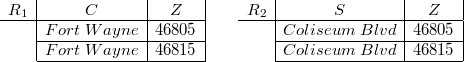
In this case  and
and  satisfy the dependencies prescribed for them separately, however in
  the dependency
  does not hold.
It is true as well, that none of the decompositions of this schema preserves the dependency  . Indeed, this is the only dependency that contains
  on the right hand side, thus if it is to be preserved, then there has to be a subschema that contains
  , but then the decomposition would not be proper. This will be considered again when decomposition into normal forms is treated.
Note that it may happen that decomposition  preserves functional dependencies, but does not have the lossless join property. Indeed, let
  ,
, 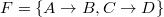 , and let the decomposition be
  .
.
Theoretically it is very simple to check whether a decomposition  is dependency preserving. Just
  needs to be calculated, then projections need to be taken, finally one should check whether the union of the projections is equivalent with
  . The main problem with this approach is that even calculating
  may need exponential time.
Nevertheless, the problem can be solved without explicitly determining  . Let
. Let  .
.  will not be calculated, only its equivalence with
  will be checked. For this end, it needs to be decidable for all functional dependencies
  that if
  is taken with respect to
  , whether it contains
  . The trick is that
  is determined without full knowledge of
  by repeatedly taking the effect to the closure of the projections of
  onto the individual
  's. That is, the concept of
  -operation on an attribute set
  is introduced, where
  is another set of attributes:
  is replaced by
  , where the closure is taken with respect to
  . Thus, the closure of the part of
  that lies in
  is taken with respect to
  , then from the resulting attributes those are added to
  , which also belong to
  .
.
It is clear that the running time of algorithm Preserve(
) is polynomial in the length of the input. More precisely, the outermost fOR loop is executed at most once for each dependency in  (it may happen that it turns out earlier that some dependency is not preserved). The body of the
 rEPEAT–uNTIL loop in lines 3–7. requires linear number of steps, it is executed at most  times. Thus, the body of the
 fOR loop needs quadratic time, so the total running time can be bounded by the cube of the input length.
Preserve(
)
1FORall2
DO3
REPEAT45
FOR
TO6
DO7
UNTIL8
IF9
THENRETURN“Not dependency preserving” 10RETURN“Dependency preserving”
Example 18.7 Consider the schema  , let the decomposition be
  , and dependencies be
  . That is, by the visible cycle of the dependencies, every attribute determines all others. Since
  and
and  do not occur together in the decomposition one might think that the dependency
  is not preserved, however this intuition is wrong. The reason is that during the projection to
  , not only the dependency
  is obtained, but
  , as well, since not
  , but
, but  is projected. Similarly,
  and
and  are obtained, as well, but
  is a logical implication of these by the transitivity of the Armstrong axioms. Thus it is expected that
 Preserve(
) claims that  is preserved.
Start from the attribute set  . There are three possible operations, the
  -operation, the
  -operation and the
  -operation. The first two obviously does not add anything to
  , since
  , that is the closure of the empty set should be taken, which is empty (in the present example). However, using the
  -operation:
In the next round using the  -operation the actual
  is changed to
  , finally applying the
  -operation on this,
  is obtained. This cannot change, so procedure
 Preserve(
) stops. Thus, with respect to the family of functional dependencies

 holds, that is
  . It can be checked similarly that the other dependencies of
  are in
  (as a fact in
  ).
).
Theorem 18.16 The procedure Preserve(
) determines correctly whether the decomposition  is dependency preserving.
Proof. It is enough to check for a single functional dependency  whether whether the procedure decides correctly if it is in
  . When an attribute is added to
  in lines 3–7, then Functional dependencies from
  are used, thus by the soundness of the Armstrong-axioms if
 Preserve(
) claims that  , then it is indeed so.
On the other hand, if  , then
 Linear-closure(
) (run by  as input) adds the attributes of
  one-by-one to
  . In every step when an attribute is added, some functional dependency
  of
of  is used. This dependency is in one of
  's, since
  is the union of these. An easy induction on the number of functional dependencies used in procedure
 Linear-closure(
) shows that sooner or later  becomes a subset of
  , then applying the
  -operation all attributes of
  are added to
  .
.
The goal of transforming (decomposing) relational schemata into normal forms is to avoid the anomalies described in the previous section. Normal forms of many different strengths were introduced in the course of evolution of database theory, here only the Boyce–Codd normal formát (BCNF) and the third, furthermore fourth normal form (3NF and 4NF) are treated in detail, since these are the most important ones from practical point of view.
Definition 18.17 Let  be relational schema,
  be a family of functional dependencies over
  .
.  is said to be in Boyce-Codd normal form if
  and
and  implies that
  is a superkey.
The most important property of BCNF is that it eliminates redundancy. This is based on the following theorem whose proof is left to the Reader as an exercise (Exercise 18.2-8).
Theorem 18.18 Schema  is in BCNF iff for arbitrary attribute
  and key
  there exists no
  , for which
  ;
;  ;
;  and
and  .
.
In other words, Theorem 18.18 states that “BCNF  There is no transitive dependence on keys”. Let us assume that a given schema is not in BCNF, for example
  and
and  hold, but
  does not, then the same
  value could occur besides many different
  values, but at each occasion the same
  value would be stored with it, which is redundant. Formulating somewhat differently, the meaning of BCNF is that (only) using functional dependencies an attribute value in a row cannot be predicted from other attribute values. Indeed, assume that there exists a schema
  , in which the value of an attribute can be determined using a functional dependency by comparison of two rows. That is, there exists two rows that agree on an attribute set
  , differ on the set
  and the value of the remaining (unique) attribute
  can be determined in one of the rows from the value taken in the other row.

If the value ? can be determined by a functional dependency, then this value can only be  , the dependency is
  , where
  is an appropriate subset of
  . However,
  cannot be a superkey, since the two rows are distinct, thus
  is not in BCNF.
Although BCNF helps eliminating anomalies, it is not true that every schema can be decomposed into subschemata in BCNF so that the decomposition is dependency preserving. As it was shown in Example 18.6, no proper decomposition of schema  preserves the
  dependency. At the same time, the schema is clearly not in BCNF, because of the
  dependency.
Since dependency preserving is important because of consistency checking of a database, it is practical to introduce a normal form that every schema has dependency preserving decomposition into that form, and it allows minimum possible redundancy. An attribute is called prime attribute, if it occurs in a key.
Definition 18.19 The schema  is in third normal form, if whenever
  , then either
  is a superkey, or
  is a prime attribute.
The schema  of Example 18.3 with the dependencies
  and
and  is not in 3NF, since
  is the only key and so
  is not a prime attribute. Thus, functional dependency
  violates the 3NF property.
3NF is clearly weaker condition than BCNF, since “or  is a prime attribute” occurs in the definition. The schema
  in Example 18.6 is trivially in 3NF, because every attribute is prime, but it was already shown that it is not in BCNF.
Theoretically every functional dependency in  should be checked whether it violates the conditions of BCNF or 3NF, and it is known that
  can be exponentially large in the size of
  . Nevertheless, it can be shown that if the functional dependencies in
  are of the form that the right hand side is a single attribute always, then it is enough to check violation of BCNF, or 3NF respectively, for dependencies of
  . Indeed, let
  be a dependency that violates the appropriate condition, that is
  is not a superkey and in case of 3NF,
  is not prime.
  . In the step when
 Closure(
) puts  into
into  (line 8) it uses a functional dependency
  from
from  that
that  and
and  . This dependency is non-trivial and
  is (still) not prime. Furthermore, if
  were a superkey, than by
  ,
,  would also be a superkey. Thus, the functional dependency
  from
from  violates the condition of the normal form. The functional dependencies easily can be checked in polynomial time, since it is enough to calculate the closure of the left hand side of each dependency. This finishes checking for BCNF, because if the closure of each left hand side is
  , then the schema is in BCNF, otherwise a dependency is found that violates the condition. In order to test 3NF it may be necessary to decide about an attribute whether it is prime or not. However this problem is NP-complete, see Problem 18-4.
Let  be a relational schema (where
  is the set of functional dependencies). The schema is to be decomposed into union of subschemata
  , such that the decomposition has the lossless join property, furthermore each
  endowed with the set of functional dependencies
  is in BCNF. The basic idea of the decomposition is simple:
-
If
 is in BCNF, then ready.
 -
If not, it is decomposed into two proper parts
 , whose join is lossless.
 -
Repeat the above for
 and
and  .
.
In order to see that this works one has to show two things:
-
If
 is not in BCNF, then it has a lossless join decomposition into smaller parts.
 -
If a part of a lossless join decomposition is further decomposed, then the new decomposition has the lossless join property, as well.
Lemma 18.20 Let  be a relational schema (where
  is the set of functional dependencies),
  be a lossless join decomposition of
  . Furthermore, let
  be a lossless join decomposition of
  with respect to
  . Then
  is a lossless join decomposition of
  .
.
The proof of Lemma 18.20 is based on the associativity of natural join. The details are left to the Reader (Exercise 18.2-9).
This can be applied for a simple, but unfortunately exponential time algorithm that decomposes a schema into subschemata of BCNF property. The projections in lines 4–5 of Naive-BCNF  may be of exponential size in the length of the input. In order to decompose schema
  , the procedure must be called with parameters
  . Procedure
 Naive-BCNF  is recursive,
  is the actual schema with set of functional dependencies
  . It is assumed that the dependencies in
  are of the form
  , where
  is a single attribute.
Naive-BCNF(
)
1WHILEthere exists, that violates BCNF 2
DO3
4
5
6
RETURN(Naive-BCNF(), Naive-BCNF}())7RETURN


However, if the algorithm is allowed overdoing things, that is to decompose a schema even if it is already in BCNF, then there is no need for projecting the dependencies. The procedure is based on the following two lemmae.
-
A schema of only two attributes is in BCNF.
-
If
 is not in BCNF, then there exists two attributes
  and
and  in
in  , such that
  holds.
Proof. If the schema consists of two attributes,  , then there are at most two possible non-trivial dependencies,
  and
and  . It is clear, that if some of them holds, then the left hand side of the dependency is a key, so the dependency does not violate the BCNF property. However, if none of the two holds, then BCNF is trivially satisfied.
On the other hand, let us assume that the dependency  violates the BCNF property. Then there must exists an attribute
  , since otherwise
  would be a superkey. For this
  ,
,  holds.
Let us note, that the converse of the second statement of Lemma 18.21 is not true. It may happen that a schema  is in BCNF, but there are still two attributes
  that satisfy
  . Indeed, let
  ,
,  . This schema is obviously in BCNF, nevertheless
  .
.
The main contribution of Lemma 18.21 is that the projections of functional dependencies need not be calculated in order to check whether a schema obtained during the procedure is in BCNF. It is enough to calculate  for pairs
  of attributes, which can be done by
 Linear-closure(
) in linear time, so the whole checking is polynomial (cubic) time. However, this requires a way of calculating  without actually projecting down the dependencies. The next lemma is useful for this task.
Lemma 18.22 Let  and let
  be the set of functional dependencies of scheme
  . Then
The proof is left for the Reader (Exercise 18.2-10). The method of lossless join BCNF decomposition is as follows. Schema  is decomposed into two subschemata. One is
  that is in BCNF, satisfying
  . The other subschema is
  , hence by Theorem 18.14 the decomposition has the lossless join property. This is applied recursively to
  , until such a schema is obtained that satisfies property 2 of Lemma 18.21. The lossless join property of this recursively generated decomposition is guaranteed by Lemma 18.20.
Polynomial-BCNF(
)
12

is the schema that is not known to be in BCNF during the procedure. 3
4
WHILEthere existin
, such that
AND5
DOLetand
be such a pair 6
7
8
WHILEthere existin
, such that
9
DO10
11
12
13
14
RETURN
The running time of Polynomial-BCNF(
) is polynomial, in fact it can be bounded by  , as follows. During each execution of the loop in lines 4–12 the size of
  is decreased by at least one, so the loop body is executed at most
  times.
  is calculated in line 4 for at most
  pairs that can be done in linear time using
 Linear-closure that results in  steps for each execution of the loop body. In lines 8–10 the size of
  is decreased in each iteration, so during each execution of lines 3–12, they give at most
  iteration. The condition of the command
 wHILE of line 8 is checked for  pairs of attributes, each checking is done in linear time. The running time of the algorithm is dominated by the time required by lines 8–10 that take
  steps altogether.
We have seen already that its is not always possible to decompose a schema into subschemata in BCNF so that the decomposition is dependency preserving. Nevertheless, if only 3NF is required then a decomposition can be given using Minimal-Cover(
). Let  be a relational schema and
  be the set of functional dependencies. Using
 Minimal-Cover(
) a minimal cover  of
of  is constructed. Let
  .
.
Theorem 18.23 The decomposition  is dependency preserving decomposition of
  into subschemata in 3NF.
Proof. Since  and the functional dependency
  is in
is in  , the decomposition preserves every dependency of
  . Let us suppose indirectly, that the schema
  is not in 3NF, that is there exists a dependency
  that violates the conditions of 3NF. This means that the dependency is non-trivial and
  is not a superkey in
  and
and  is not a prime attribute of
  . There are two cases possible. If
  , then using that
  is not a superkey
  follows. In this case the functional dependency
  contradicts to that
  was a member of minimal cover, since its left hand side could be decreased. In the case when
  ,
,  holds.
  is not prime in
  , thus
  is not a key, only a superkey. However, then
  would contain a key
  such that
  . Furthermore,
  would hold, as well, that contradicts to the minimality of
  since the left hand side of
  could be decreased.
If the decomposition needs to have the lossless join property besides being dependency preserving, then  given in Theorem 18.23 is to be extended by a key
  of
of  . Although it was seen before that it is not possible to list all keys in polynomial time, one can be obtained in a simple greedy way, the details are left to the Reader (Exercise 18.2-11).
Theorem 18.24 Let  be a relational schema, and let
  be a minimal cover of
  . Furthermore, let
  be a key in
  . Then the decomposition
  is a lossless join and dependency preserving decomposition of
  into subschemata in 3NF.
Proof. It was shown during the proof of Theorem 18.23 that the subschemata  are in 3NF for
  . There cannot be a non-trivial dependency in the subschema
  , because if it were, then
  would not be a key, only a superkey.
The lossless join property of  is shown by the use of
 Join-test(
) procedure. Note that it is enough to consider the minimal cover  of
of  . More precisely, we show that the row corresponding to
  in the table will be all 0 after running
 Join-test(
). Let  be the order of the attributes of
  as
as Closure(
) inserts them into  . Since
  is a key, every attribute of
  is taken during
 Closure(
). It will be shown by induction on  that the element in row of
  and column of
  is 0 after running
 Join-test(
).
The base case of  is obvious. Let us suppose that the statement is true for
  and consider when and why
  is inserted into
  . In lines 6–8 of
 Closure(
) such a functional dependency  is used where
  . Then
  ,
,  for some
  . The rows corresponding to
  and
and  agree in columns of
  (all 0 by the induction hypothesis), thus the entries in column of
  are equated by
 Join-test(
). This value is 0 in the row corresponding to  , thus it becomes 0 in the row of
  , as well.
It is interesting to note that although an arbitrary schema can be decomposed into subschemata in 3NF in polynomial time, nevertheless it is NP-complete to decide whether a given schema  is in 3NF, see Problem 18-4. However, the BCNF property can be decided in polynomial time. This difference is caused by that in order to decide 3NF property one needs to decide about an attribute whether it is prime. This latter problem requires the listing of all keys of a schema.
Example 18.8 Besides functional dependencies, some other dependencies hold in Example 18.1, as well. There can be several lectures of a subject in different times and rooms. Part of an instance of the schema could be the following.
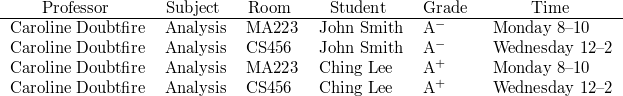
A set of values of Time and Room attributes, respectively, belong to each given value of Subject, and all other attribute values are repeated with these. Sets of attributes SR and StG are independent, that is their values occur in each combination.
The set of attributes  is said to be multivalued dependent on set of attributes
  , in notation
  , if for every value on
  , there exists a set of values on
  that is not dependent in any way on the values taken in
  . The precise definition is as follows.
Definition 18.25 The relational schema  satisfies the multivalued dependency
  , if for every relation
  of schema
  and arbitrary tuples
  of
of  that satisfy
  , there exists tuples
  such that


holds.
Footnote. It would be enough to require the existence of  , since the existence of
  would follow. However, the symmetry of multivalued dependency is more apparent in this way.
In Example 18.8 S  TR holds.
Remark 18.26 Functional dependency is equality generating dependency, that is from the equality of two objects it deduces the equality of other other two objects. On the other hand, multivalued dependency is tuple generating dependency, that is the existence of two rows that agree somewhere implies the existence of some other rows.
There exists a sound and complete axiomatisation of multivalued dependencies similar to the Armstrong-axioms of functional dependencies. Logical implication and inference can be defined analogously. The multivalued dependency  is logically implied by the set
  of multivalued dependencies, in notation
  , if every relation that satisfies all dependencies of
  also satisfies
  .
.
Note, that  implies
  . The rows
  and
and  of Definition 18.25 can be chosen as
  and
and  , respectively. Thus, functional dependencies and multivalued dependencies admit a common axiomatisation. Besides Armstrong-axioms (A1)–(A3), five other are needed. Let
  be a relational schema.
-
(A4) Complementation:
 .
. -
(A5) Extension: If
 holds, and
  , then
  .
. -
(A6) Transitivity:
 .
. -
(A7)
 .
. -
(A8) If
 holds,
  , furthermore for some
  disjoint from
 holds, then
  is true, as well.
Beeri, Fagin and Howard proved that (A1)–(A8) is sound and complete system of axioms for functional and Multivalued dependencies together. Proof of soundness is left for the Reader (Exercise 18.2-12), the proof of the completeness exceeds the level of this book. The rules of Lemma 18.2 are valid in exactly the same way as when only functional dependencies were considered. Some further rules are listed in the next Proposition.
Claim 18.27 The followings are true for multivalued dependencies.
-
Union rule:
 .
. -
Pseudotransitivity:
 .
. -
Mixed pseudotransitivity:
 .
. -
Decomposition rule for multivalued dependencies: if
 and
and  holds, then
  ,
,  and
and  holds, as well.
The proof of Proposition 18.27 is left for the Reader (Exercise 18.2-13).
Important difference between functional dependencies and multivalued dependencies is that  immediately implies
  for all
  in
in  , however
  is deduced by the decomposition rule for multivalued dependencies from
  only if there exists a set of attributes
  such that
  and
and  , or
, or  . Nevertheless, the following theorem is true.
Theorem 18.28 Let  be a relational schema,
  be a set of attributes. Then there exists a partition
  of the set of attributes
  such that for
  the multivalued dependency
  holds if and only if
  is the union of some
  's.
's.
Proof. We start from the one-element partition  . This will be refined successively, while the property that
  holds for all
  in the actual decomposition, is kept. If
  and
and  is not a union of some of the
  's, then replace every
  such that neither
  nor
nor  is empty by
  and
and  . According to the decomposition rule of Proposition 18.27, both
  and
and  hold. Since
  is finite, the refinement process terminates after a finite number of steps, that is for all
  such that
  holds,
  is the union of some blocks of the partition. In order to complete the proof one needs to observe only that by the union rule of Proposition 18.27, the union of some blocks of the partition depends on
  in multivalued way.
Definition 18.29 The partition  constructed in Theorem 18.28 from a set
  of functional and multivalued dependencies is called the dependency basis of
  (with respect to
  ).
).
Example 18.9 Consider the familiar schema
| R(Professor,Subject,Room,Student,Grade,Time) |
of Examples 18.1 and 18.8. Su  RT was shown in Example 18.8. By the complementation rule Su
  PStG follows. Su
  P is also known. This implies by axiom (A7) that Su
  P. By the decomposition rule Su
  Stg follows. It is easy to see that no other one-element attribute set is determined by Su via multivalued dependency. Thus, the dependency basis of Su is the partition {P,RT,StG}.
We would like to compute the set  of logical consequences of a given set
  of functional and multivalued dependencies. One possibility is to apply axioms (A1)–(A8) to extend the set of dependencies repeatedly, until no more extension is possible. However, this could be an exponential time process in the size of
  . One cannot expect any better, since it was shown before that even
  can be exponentially larger than
  . Nevertheless, in many applications it is not needed to compute the whole set
  , one only needs to decide whether a given functional dependency
  or multivalued dependency
  belongs to
  or not. In order to decide about a multivalued dependency
  , it is enough to compute the dependency basis of
  , then to check whether
  can be written as a union of some blocks of the partition. The following is true.
Theorem 18.30 (Beeri) In order to compute the dependency basis of a set of attributes  with respect to a set of dependencies
  , it is enough to consider the following set
  of multivalued dependencies:
-
All multivalued dependencies of
 and
and -
for every
 in
in  the set of multivalued dependencies
  , where
  , and the
  's are single attributes.
The only thing left is to decide about functional dependencies based on the dependency basis. Closure(
) works correctly only if multivalued dependencies are not considered. The next theorem helps in this case.
Theorem 18.31 (Beeri) Let us assume that  and the dependency basis of
  with respect to the set
  of multivalued dependencies obtained in Theorem 18.30 is known.
  holds if and only if
-
 forms a single element block in the partition of the dependency basis, and
 -
There exists a set
 of attributes that does not contain
  ,
,  is an element of the originally given set of dependencies
  , furthermore
  .
.
Based on the observations above, the following polynomial time algorithm can be given to compute the dependency basis of a set of attributes  .
.
Dependency-Basis(
)
1
The collection of sets in the dependency basis is
. 2
REPEAT3FORall4
DOIFthere existssuch that
5
THEN6
UNTILdoes not change 7
RETURN

It is immediate that if  changes in lines 3–5. of
 Dependency-basis(
), then some block of the partition is cut by the algorithm. This implies that the running time is a polynomial function of the sizes of  and
and  . In particular, by careful implementation one can make this polynomial to
  , see Problem 18-5.
The Boyce-Codd normal form can be generalised to the case where multivalued dependencies are also considered besides functional dependencies, and one needs to get rid of the redundancy caused by them.
Definition 18.32 Let  be a relational schema,
  be a set of functional and multivalued dependencies over
  .
.  is in fourth normal form (4NF), if for arbitrary multivalued dependency
  for which
  and
and  , holds that
  is superkey in
  .
.
Observe that 4NF  BCNF. Indeed, if
  violated the BCNF condition, then
  , furthermore
  could not contain all attributes of
  , because that would imply that
  is a superkey. However,
  implies
  by (A8), which in turn would violate the 4NF condition.
Schema  together with set of functional and multivalued dependencies
  can be decomposed into
  , where each
  is in 4NF and the decomposition has the lossless join property. The method follows the same idea as the decomposition into BCNF subschemata. If schema
  is not in 4NF, then there exists a multivalued dependency
  in the projection of
  onto
onto  that violates the 4NF condition. That is,
  is not a superkey in
  ,
,  neither is empty, nor is a subset of
  , furthermore the union of
  and
and  is not
  . It can be assumed without loss of generality that
  and
and  are disjoint, since
  is implied by
  using (A1), (A7) and the decomposition rule. In this case
  can be replaced by subschemata
  and
and  , each having a smaller number of attributes than
  itself, thus the process terminates in finite time.Two things has to be dealt with in order to see that the process above is correct.
-
Decomposition
 has the lossless join property.
 -
How can the projected dependency set
 be computed?
 -
The first problem is answered by the following theorem.
Theorem 18.33 The decomposition  of schema
  has the lossless join property with respect to a set of functional and multivalued dependencies
  iff
iff
Proof. The decomposition  of schema
  has the lossless join property iff for any relation
  over the schema
  that satisfies all dependencies from
  holds that if
  and
and  are two tuples of
  , then there exists a tuple
  satisfying
  and
and  , then it is contained in
  . More precisely,
  is the natural join of the projections of
  on
on  and of
  on
on  , respectively, which exist iff
  . Thus the fact that
  is always contained in
  is equivalent with that
  .
.
To compute the projection  of the dependency set
  one can use the following theorem of Aho, Beeri and Ullman.
  is the set of multivalued dependencies that are logical implications of
  and use attributes of
  only.
only.
Theorem 18.34 (Aho, Beeri és Ullman)  consists of the following dependencies:
-
For all
 , if
, if  , then
  .
. -
For all
 , if
, if  , then
  .
.
Other dependencies cannot be derived from the fact that  holds in
  .
.
Unfortunately this theorem does not help in computing the projected dependencies in polynomial time, since even computing  could take exponential time. Thus, the algorithm of 4NF decomposition is not polynomial either, because the 4NF condition must be checked with respect to the projected dependencies in the subschemata. This is in deep contrast with the case of BCNF decomposition. The reason is, that to check BCNF condition one does not need to compute the projected dependencies, only closures of attribute sets need to be considered according to Lemma 18.21.
Exercises
18.2-1 Are the following inference rules sound?
a. If  and
and  , then
  .
.
b. If  and
and  , then
  .
.
c. If  and
and  , then
  .
.
18.2-2 Prove Theorem 18.30, that is show the following. Let  be a set of functional and multivalued dependencies, and let
  . Then
a.  , and
, and
b.  .
.
Hint. Use induction on the inference rules to prove b.
18.2-3 Consider the database of an investment firm, whose attributes are as follows:  (stockbroker),
  (office of stockbroker),
  (investor),
  (stock),
  (amount of stocks of the investor),
  (dividend of the stock). The following functional dependencies are valid:
  ,
,  ,
,  ,
,  .
.
a. Determine a key of schema  .
.
b. How many keys are in schema  ?
?
c. Give a lossless join decomposition of  into subschemata in BCNF.
d. Give a dependency preserving and lossless join decomposition of  into subschemata in 3NF.
18.2-4 The schema  of Exercise 18.2-3 is decomposed into subschemata
  ,
,  ,
,  and
and  . Does this decomposition have the lossless join property?
18.2-5 Assume that schema  of Exercise 18.2-3 is represented by
  ,
,  ,
,  and
and  subschemata. Give a minimal cover of the projections of dependencies given in Exercise 18.2-3. Exhibit a minimal cover for the union of the sets of projected dependencies. Is this decomposition dependency preserving?
18.2-6 Let the functional dependency  of Exercise 18.2-3 be replaced by the multivalued dependency
  . That is ,
  represents the stock's dividend “history”.
a. Compute the dependency basis of  .
.
b. Compute the dependency basis of  .
.
c. Give a decomposition of  into subschemata in 4NF.
18.2-7 Consider the decomposition  of schema
  . Let
. Let  , furthermore
  . Prove:
a.  .
.
b. If  , then
  .
.
c.  .
.
18.2-8 Prove that schema  is in BCNF iff for arbitrary
  and key
  , it holds that there exists no
  , for which
  ;
;  ;
;  and
and  .
.
18.2-9 Prove Lemma 18.20.
18.2-10 Let us assume that  and the set of functional dependencies of schema
  is
is  . Prove that
  .
.
18.2-11 Give a  running time algorithm to find a key of the relational schema
  .
.
Hint. Use that  is superkey and each superkey contains a key. Try to drop attributes from
  one-by-one and check whether the remaining set is still a key.
18.2-12 Prove that axioms (A1)–(A8) are sound for functional and multivalued dependencies.
18.2-13 Derive the four inference rules of Proposition 18.27 from axioms (A1)–(A8).
Two such dependencies will be discussed in this section that are generalizations of the previous ones, however cannot be axiomatised with axioms similar to (A1)–(A8).
Theorem 18.33 states that multivalued dependency is equivalent with that some decomposition the schema into two parts has the lossless join property. Its generalisation is the join dependency.
Definition 18.35 Let  be a relational schema and let
  . The relation
  belonging to
  is said to satisfy the join dependency
if
In this setting  satisfies multivalued dependency
  iff it satisfies the join dependency
  . The join dependency
  expresses that the decomposition
  has the lossless join property. One can define the fifth normal form, 5NF.
Definition 18.36 The relational schema  is in fifth normal form, if it is in 4NF and has no non-trivial join dependency.
The fifth normal form has theoretical significance primarily. The schemata used in practice usually have primary keys. Using that the schema could be decomposed into subschemata of two attributes each, where one of the attributes is a superkey in every subschema.
Example 18.10 Consider the database of clients of a bank (Client-number,Name,Address,accountBalance). Here C is unique identifier, thus the schema could be decomposed into (CN,CA,CB), which has the lossless join property. However, it is not worth doing so, since no storage place can be saved, furthermore no anomalies are avoided with it.
There exists an axiomatisation of a dependency system if there is a finite set of inference rules that is sound and complete, i.e. logical implication coincides with being derivable by using the inference rules. For example, the Armstrong-axioms give an axiomatisation of functional dependencies, while the set of rules (A1)–(A8) is the same for functional and multivalued dependencies considered together. Unfortunately, the following negative result is true.
Theorem 18.37 The family of join dependencies has no finite axiomatisation.
In contrary to the above, Abiteboul, Hull and Vianu show in their book that the logical implication problem can be decided by an algorithm for the family of functional and join dependencies taken together. The complexity of the problem is as follows.
-
It is NP-complete to decide whether a given join dependency is implied by another given join dependency and a functional dependency.
-
It is NP-hard to decide whether a given join dependency is implied by given set of multivalued dependencies.
A generalisation of functional dependencies is the family of branching dependencies. Let us assume that  and there exists no
  rows in relation
  over schema
  , such that they contain at most
  distinct values in columns of
  , but all
  values are pairwise distinct in some column of
  . Then
  is said to be
  -dependent on
  , in notation
  . In particular,
  holds if and only if functional dependency
  holds.
Example 18.11 Consider the database of the trips of an international transport truck.
-
One trip: four distinct countries.
-
One country has at most five neighbours.
-
There are 30 countries to be considered.
Let  be the attributes of the countries reached in a trip. In this case
  does not hold, however another dependency is valid:

The storage space requirement of the database can be significantly reduced using these dependencies. The range of each element of the original table consists of 30 values, names of countries or some codes of them (5 bits each, at least). Let us store a little table ( bits) that contains a numbering of the neighbours of each country, which assigns to them the numbers 0,1,2,3,4 in some order. Now we can replace attribute
  by these numbers (
 ), because the value of
  gives the starting country and the value of
  determines the second country with the help of the little table. The same holds for the attribute
  , but we can decrease the number of possible values even further, if we give a table of numbering the possible third countries for each
  pair. In this case, the attribute
  can take only 4 different values. The same holds for
  , too. That is, while each element of the original table could be encoded by 5 bits, now for the cost of two little auxiliary tables we could decrease the length of the elements in the second column to 3 bits, and that of the elements in the third and fourth columns to 2 bits.
The  -closure of an attribute set
  can be defined:

In particular,  . In case of branching dependencies even such basic questions are hard as whether there exists an Armstrong-relation for a given family of dependencies.
Definition 18.39 Let  be a relational schema,
  be a set of dependencies of some dependency family
  defined on
  . A relation
  over schema
  is Armstrong-relation for
  , if the set of dependencies from
  that
that  satisfies is exactly
  , that is
  .
.
Armstrong proved that for an arbitrary set of functional dependencies  there exists Armstrong-relation for
  . The proof is based on the three properties of closures of attributes sets with respect to
  , listed in Exercise 18.1-1. For branching dependencies only the first two holds in general.
Lemma 18.40 Let  , furthermore let
  be a relational schema. For
  one has
-
 and
and -
 .
.
There exists such  mapping and natural numbers
  that there exists no Armstrong-relation for
  in the family if
  -dependencies.Grant Minker investigated numerical dependencies that are similar to branching dependencies. For attribute sets
  the dependency
  holds in a relation
  over schema
  if for every tuple value taken on the set of attributes
  , there exists at most
  distinct tuple values taken on
  . This condition is stronger than that of
  , since the latter only requires that in each column of
  there are at most
  values, independently of each other. That allows
  different
  projections. Numerical dependencies were axiomatised in some special cases, based on that Katona showed that branching dependencies have no finite axiomatisation. It is still an open problem whether logical implication is algorithmically decidable amongst branching dependencies.
Exercises
18.3-1 Prove Theorem 18.38.
18.3-2 Prove Lemma 18.40.
18.3-3 Prove that if  , then
  holds besides the two properties of Lemma 18.40.
18.3-4 A  mapping is called a closure, if it satisfies the two properties of Lemma 18.40 and and the third one of Exercise 18.3-3. Prove that if
  is a closure, and
  is the family of dependencies defined by
  , then there exists an Armstrong-relation for
  in the family of
  -dependencies (functional dependencies) and in the family of
  -dependencies, respectively.
18.3-5 Let  be the closure defined by
Prove that there exists no Armstrong-relation for  in the family of
  -dependencies, if
  .
.
PROBLEMS |
18-1 External attributes
Maier calls attribute  an external attribute in the functional dependency
  with respect to the family of dependencies
  over schema
  , if the following two conditions hold:
-
 , or
, or -
 .
.
Design an  running time algorithm, whose input is schema
  and output is a set of dependencies
  equivalent with
  that has no external attributes.
18-2 The order of the elimination steps in the construction of minimal cover is important
In the procedure Minimal-cover(
) the set of functional dependencies was changed in two ways: either by dropping redundant dependencies, or by dropping redundant attributes from the left hand sides of the dependencies. If the latter method is used first, until there is no more attribute that can be dropped from some left hand side, then the first method, this way a minimal cover is obtained really, according to Proposition 18.6. Prove that if the first method applied first and then the second, until there is no more possible applications, respectively, then the obtained set of dependencies is not necessarily a minimal cover of  .
.
18-3 BCNF subschema
Prove that the following problem is coNP-complete: Given a relational schema  with set of functional dependencies
  , furthermore
  , decide whether
  is in BCNF.
Let  be a relational schema, where
  is the system of functional dependencies.
The  size key problem is the following: given a natural number
  , determine whether there exists a key of size at most
  .
.
The prime attribute problem is the following: for a given  , determine whether it is a prime attribute.
-
a. Prove that the
 size key problem is NP-complete. Hint. Reduce the vertex cover problem to the prime attribute problem.
 -
b. Prove that the prime attribute problem is NP-complete by reducing the
 size key problem to it.
 -
c. Prove that determining whether the relational schema
 is in 3NF is NP-complete. Hint. Reduce the prime attribute problem to it.
18-5 Running time of Dependency-basis
Give an implementation of procedure Dependency-basis, whose running time is  .
.
CHAPTER NOTES |
The relational data model was introduced by Codd [66] in 1970. Functional dependencies were treated in his paper of 1972 [70], their axiomatisation was completed by Armstrong [20]. The logical implication problem for functional dependencies were investigated by Beeri and Bernstein [32], furthermore Maier [232]. Maier also treats the possible definitions of minimal covers, their connections and the complexity of their computations in that paper. Maier, Mendelzon and Sagiv found method to decide logical implications among general dependencies [233]. Beeri, Fagin and Howard proved that axiom system (A1)–(A8) is sound and complete for functional and multivalued dependencies taken together [34]. Yu and Johnson [353] constructed such relational schema, where  and the number of keys is
  . Békéssy and Demetrovics [42] gave a simple and beautiful proof for the statement, that from
  functional dependencies at most
  keys can be obtained, thus Yu and Johnson's construction is extremal.
Armstrong-relations were introduced and studied by Fagin [100], [101], furthermore by Beeri, Fagin, Dowd and Statman [33].
Multivalued dependencies were independently discovered by Zaniolo [356], Fagin [102] and Delobel [83].
The necessity of normal forms was recognised by Codd while studying update anomalies [68], [67]. The Boyce–Codd normal form was introduced in [69]. The definition of the third normal form used in this chapter was given by Zaniolo [357]. Complexity of decomposition into subschemata in certain normal forms was studied by Lucchesi and Osborne [225], Beeri and Bernstein [32], furthermore Tsou and Fischer [328].
Theorems 18.30 and 18.31 are results of Beeri [31]. Theorem 18.34 is from a paper of Aho, Beeri és Ullman [6].
Theorems 18.37 and 18.38 are from the book of Abiteboul, Hull and Vianu [3], the non-existence of finite axiomatisation of join dependencies is Petrov's result [271].
Branching dependencies were introduced by Demetrovics, Katona and Sali, they studied existence of Armstrong-relations and the size of minimal Armstrong-relations [84], [85], [86], [292]. Katona showed that there exists no finite axiomatisation of branching dependencies in (ICDT'92 Berlin, invited talk) but never published.
Possibilities of axiomatisation of numerical dependencies were investigated by Grant and Minker [142], [143].
Good introduction of the concepts of this chapter can be found in the books of Abiteboul, Hull and Vianu [3], Ullman [331] furthermore Thalheim [321], respectively.
Table of Contents
In chapter “Relational database design” basic concepts of relational databases were introduced, such as relational schema, relation, instance. Databases were studied from the designer point of view, the main question was how to avoid redundant data storage, or various anomalies arising during the use of the database.
In the present chapter the schema is considered to be given and focus is on fast and efficient ways of answering user queries. First, basic (theoretical) query languages and their connections are reviewed in Section 19.1.
In the second part of this chapter (Section 19.2) views are considered. Informally, a view is nothing else, but result of a query. Use of views in query efficiency, providing physical data independence and data integration is explained.
Finally, the third part of the present chapter (Section 19.3) introduces query rewriting.
Consider the database of cinemas in Budapest. Assume that the schema consists of three relations:

The schemata of individual relations are as follows:

Possible values of instances of each relation are shown on Figure 19.1.
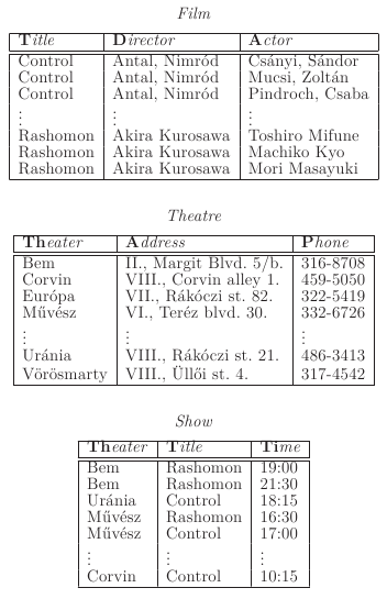
Typical user queries could be:
-
19.1 Who is the director of “Control”?
-
19.2 List the names address of those theatres where Kurosawa films are played.
-
19.3 Give the names of directors who played part in some of their films.
These queries define a mapping from the relations of database schema CinePest to some other schema (in the present case to schemata of single relations). Formally, query and query mapping should be distinguished. The former is a syntactic concept, the latter is a mapping from the set of instances over the input schema to the set of instances over the output schema, that is determined by the query according to some semantic interpretation. However, for both concepts the word “query” is used for the sake of convenience, which one is meant will be clear from the context.
Definition 19.1 Queries  and
and  over schema
  are said to be equivalent, in notation
  , if they have the same output schema and for every instance
  over schema
 holds.
In the remaining of this chapter the most important query languages are reviewed. The expressive powers of query languages need to be compared.
Definition 19.2 Let  and
and  be query languages (with appropriate semantics).
  is dominated by
  (
( is weaker, than
  ), in notation
  , if for every query
  of
of  there exists a query
  , such that
  .
.  and
and  are equivalent, if
  and
and  .
.
Example 19.1 Query. Consider Question 19.2. As a first try the next solution is obtained:
-
iFthere exist in relations Film, Theater and Show tuples ,
,  and
and 
-
tHENput the tuple into the output relation.
 denote different variables that take their values from the domains of the corresponding attributes, respectively. Using the same variables implicitly marked where should stand identical values in different tuples.
Conjunctive queries are the simplest kind of queries, but they are the easiest to handle and have the most good properties. Three equivalent forms will be studied, two of them based on logic, the third one is of algebraic nature. The name comes from first order logic expressions that contain only existential quantors ( ), furthermore consist of atomic expressions connected with logical “and”, that is conjunction.
The tuple  is called free tuple if the
  's are variables or constants. This is a generalisation of a tuple of a relational instance. For example, the tuple
  in Example 19.1 is a free tuple.
Definition 19.3 Let  be a relational database schema. Rule based conjunctive query is an expression of the following form

where  ,
,  are relation names from
  ,
,  is a relation name not in
  ,
,  are free tuples. Every variable occurring in
  must occur in one of
  , as well.
The rule based conjunctive query is also called a rule for the sake of simplicity.  is the head of the rule,
  is the body of the rule,
  is called a (relational) atom. It is assumed that each variable of the head also occurs in some atom of the body.
A rule can be considered as some tool that tells how can we deduce newer and newer facts, that is tuples, to include in the output relation. If the variables of the rule can be assigned such values that each atom  is true (that is the appropriate tuple is contained in the relation
  ), then tuple
  is added to the relation
  . Since all variables of the head occur in some atoms of the body, one never has to consider infinite domains, since the variables can take values from the actual instance queried. Formally. let
  be an instance over relational schema
  , furthermore let
  be a the query given by rule (19.3). Let
  denote the set of variables occurring in
  , and let
  denote the set of constants that occur in
  . The image of
  under
under  is given by

An immediate way of calculating  is to consider all possible valuations
  in some order. There are more efficient algorithms, either by equivalent rewriting of the query, or by using some indices.
An important difference between atoms of the body and the head is that relations  are considered given, (physically) stored, while relation
  is not, it is thought to be calculated by the help of the rule. This justifies the names:
  's are extensional relations and
  is intensional relation.
Query  over schema
  is monotone, if for instances
  and
and  over
over  ,
,  implies
  .
.  is satisfiable, if there exists an instance
  , such that
  . The proof of the next simple observation is left for the Reader (Exercise 19.1-1).
Claim 19.4 Rule based queries are monotone and satisfiable.
Proposition 19.4 shows the limitations of rule based queries. For example, the query Which theatres play only Kurosawa films? is obviously not monotone, hence cannot be expressed by rules of form (19.3).
If the difference between variables and constants is not considered, then the body of a rule can be viewed as an instance over the schema. This leads to a tabular form of conjunctive queries that is most similar to the visual queries (QBE: Query By Example) of database management system Microsoft Access.
Definition 19.5 A tableau over the schema  is a generalisation of an instance over
  , in the sense that variables may occur in the tuples besides constants. The pair
  is a tableau query if
  is a tableau and
  is a free tuple such that all variables of
  occur in
  , as well. The free tuple
  is the summary.
The summary row  of tableau query
  shows which tuples form the result of the query. The essence of the procedure is that the pattern given by tableau
  is searched for in the database, and if found then the tuple corresponding to is included in the output relation. More precisely, the mapping
  is an embedding of tableau
  into instance
  , if
, if  . The output relation of tableau query
  consists of all tuples
  that
that  is an embedding of tableau
  into instance
  .
.
Example 19.2 Tableau query Let  be the following tableau.
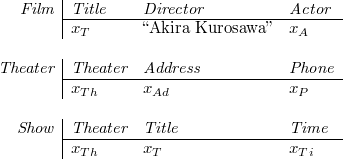
The tableau query  answers question 19.2 of the introduction.
The syntax of tableau queries is similar to that of rule based queries. It will be useful later that conditions for one query to contain another one can be easily formulated in the language of tableau queries.
 .
.A database consists of relations, and a relation is a set of tuples. The result of a query is also a relation with a given attribute set. It is a natural idea that output of a query could be expressed by algebraic and other operations on relations. The relational algebra  consists of the following operations.
Footnote. The relational algebra  is the monotone part of the (full) relational algebra introduced later.
-
Selection: It is of form either
 or
or  , where
  and
and  are attributes while
  is a constant. The operation can be applied to all such relations
  that has attribute
  (and
(and  ), and its result is relation
  that has the same set of attributes as
  has, and consists of all tuples that satisfy the selection condition.
 -
Projection: The form of the operation is
 ,
,  , where
  's are distinct attributes. It can be applied to all such relations whose attribute set includes each
  and its result is the relation
  that has attribute set
  ,
, that is it consists of the restrictions of tuples in
 to the attribute set
  .
. -
Natural join: This operation has been defined earlier in chapter “Relational database design”. Its notation is
 , its input consists of two (or more) relations
  ,
,  , with attribute sets
  ,
,  , respectively. The attribute set of the output relation is
  .
. -
Renaming: Attribute renaming is nothing else, but an injective mapping from a finite set of attributes
 into the set of all attributes. Attribute renaming
  can be given by the list of pairs
  , where
  , which is written usually in the form
  . The renaming operator
  maps from inputs over
  to outputs over
  . If
. If  is a relation over
  , then


Relational algebra  queries are obtained by finitely many applications of the operations above from relational algebra base queries, which are
-
Input relation:
 .
. -
Single constant:
 , where
  is a constant,
  is an attribute name.
Example 19.3 Relational algebra  query. The question 19.2 of the introduction can be expressed with relational algebra operations as follows.

The mapping given by a relational algebra  query can be easily defined via induction on the operation tree. It is easy to see (Exercise 19.1-2) that non-satisfiable queries can be given using relational algebra
  . There exist no rule based or tableau query equivalent with such a non-satisfiable query. Nevertheless, the following is true.
Theorem 19.6 Rule based queries, tableau queries and satisfiable relational algebra  are equivalent query languages.
The proof of Theorem 19.6 consists of three main parts:
-
Rule based
 Tableau
 -
Satisfiable relational algebra

 Rule based
 -
Rule based
 Satisfiable relational algebra
The first (easy) step is left to the Reader (Exercise 19.1-3). For the second step, it has to be seen first, that the language of rule based queries is closed under composition. More precisely, let  be a database,
  be a query over
  . If the output relation of
  is
is  , then in a subsequent query
  can be used in the same way as any extensional relation of
  . Thus relation
  can be defined, then with its help relation
  can be defined, and so on. Relations
  are intensional relations. The conjunctive query program
  is a list of rules
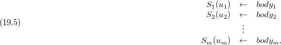
where  's are pairwise distinct and not contained in
  . In rule body
  only relations
  and
and  can occur.
  is considered to be the output relation of
  , its evaluation is is done by computing the results of the rules one-by-one in order. It is not hard to see that with appropriate renaming the variables
  can be substituted by a single rule, as it is shown in the following example.
Example 19.4 Conjunctive query program. Let  , and consider the following conjunctive query program

 can be written using
  and
and  only by the first two rules of (19.6)

It is apparent that some variables had to be renamed to avoid unwanted interaction of rule bodies. Substituting expression (19.7) into the third rule of (19.6) in place of  , and appropriately renaming the variables

is obtained.
Thus it is enough to realise each single relational algebra  operation by an appropriate rule.
-
 Let
Let  denote the list of variables (and constants) corresponding to the common attributes of
  and
and  , let
, let  denote the variables (and constants) corresponding to the attributes occurring only in
  , while
  denotes those of corresponding to
  's own attributes. Then rule
  gives exactly relation
  .
. -
 Assume that
  and the selection condition
  is of form either
  or
or  , where
  are attributes
  is constant. Then
 respectively,
are the rules sought. The satisfiability of relational algebra
 query is used here. Indeed, during composition of operations we never obtain an expression where two distinct constants should be equated.
 -
 If
If  , then
 works.
-
 The renaming operation of relational algebra
  can be achieved by renaming the appropriate variables, as it was shown in Example 19.4.


For the proof of the third step let us consider rule

By renaming the attributes of relations  's, we may assume without loss of generality that all attribute names are distinct. Then
  can be constructed that is really a direct product, since the the attribute names are distinct. The constants and multiple occurrences of variables of rule (19.9) can be simulated by appropriate selection operators. The final result is obtained by projecting to the set of attributes corresponding to the variables of relation
  .
.
Conjunctive queries are a class of query languages that has many good properties. However, the set of expressible questions are rather narrow. Consider the following.
-
19.4 List those pairs where one member directed the other member in a film, and vice versa, the other member also directed the first in a film.
-
19.5 Which theatres show “La Dolce Vita” or “Rashomon”?
-
19.6 Which are those films of Hitchcock that Hitchcock did not play a part in?
-
19.7 List those films whose every actor played in some film of Fellini.
-
19.8 Let us recall the game “Chain-of-Actors”. The first player names an actor/actress, the next another one who played in some film together with the first named. This is continued like that, always a new actor/actress has to be named who played together with the previous one. The winner is that player who could continue the chain last time. List those actors/actresses who could be reached by “Chain-of-Actors” starting with “Marcello Mastroianni”.
Question 19.4 can be easily answered if equalities are also allowed rule bodies, besides relational atoms:

Allowing equalities raises two problems. First, the result of the query could become infinite. For example, the rule based query

results in an infinite number of tuples, since variables  and
and  are not bounded by relation
  , thus there can be an infinite number of evaluations that satisfy the rule body. Hence, the concept of domain restricted query is introduced. Rule based query
  is domain restricted, if all variables that occur in the rule body also occur in some relational atom.
The second problem is that equality atoms may cause the body of a rule become unsatisfiable, in contrast to Proposition 19.4. For example, query

is domain restricted, however if  and
and  are distinct constants, then the answer will be empty. It is easy to check whether a rule based query with equality atoms is satisfiable.
Satisfiable(
)
1 Compute the transitive closure of equalities of the body of. 2
IFTwo distinct constants should be equal by transitivity 3THENRETURN“Not satisfiable.” 4ELSERETURN“Satisfiable.”
It is also true (Exercise 19.1-4) that if a rule based query  that contains equality atoms is satisfiable, then there exists a another rule based query
  without equalities that is equivalent with
  .
.
The question 19.5 cannot be expressed with conjunctive queries. However, if the union operator is added to relational algebra, then 19.5 can be expressed in that extended relational algebra:

Rule based queries are also capable of expressing question 19.5 if it is allowed that the same relation is in the head of many distinct rules:

Non-recursive datalog program is a generalisation of this.
Definition 19.7 A non-recursive datalog program over schema  is a set of rules

where no relation of  occurs in a head, the same relation may occur in the head of several rules, furthermore there exists an ordering
  of the rules such that the relation in the head of
  does not occur in the body of any rule
  for
for  .
.
The semantics of the non-recursive datalog program (19.15) is similar to the conjunctive query program (19.5). The rules are evaluated in the order  of Definition 19.7, and if a relation occurs in more than one head then the union of the sets of tuples given by those rules is taken.
The union of tableau queries 
 is denoted by
  . It is evaluated by individually computing the result of each tableau query
  , then the union of them is taken. The following holds.
Theorem 19.8 The language of non-recursive datalog programs with unique output relation and the relational algebra extended with the union operator are equivalent.
The proof of Theorem 19.8 is similar to that of Theorem 19.6 and it is left to the Reader (Exercise 19.1-5). Let us note that the expressive power of the union of tableau queries is weaker. This is caused by the requirement having the same summary row for each tableau. For example, the non-recursive datalog program query

cannot be realised as union of tableau queries.
The query 19.6 is obviously not monotone. Indeed, suppose that in relation Film there exist tuples about Hitchcock's film Psycho, for example (“Psycho”,“A. Hitchcock”,“A.Perkins”), (“Psycho”,“A. Hitchcock”,“J. Leigh”),  , however, the tuple (“Psycho”,“A.Hitchcock”,“A. Hitchcock”) is not included. Then the tuple (“Psycho”) occurs in the output of query 19.6. With some effort one can realize however, that Hitchcock appears in the film Psycho, as “a man in cowboy hat”. If the tuple (“Psycho”,“A. Hitchcock”,“A. Hitchcock”) is added to relation Film as a consequence, then the instance of schema CinePest gets larger, but the output of query 19.6 becomes smaller.
It is not too hard to see that the query languages discussed so far are monotone, hence query 19.6 cannot be formulated with non-recursive datalog program or with some of its equivalents. Nevertheless, if the difference  operator is also added to relation algebra, then it becomes capable of expressing queries of type 19.6 For example,

realises exactly query 19.6. Hence, the (full) relational algebra consists of operations  . The importance of the relational algebra is shown by the fact, that Codd calls a query language
  relationally complete, exactly if for all relational algebra query
  there exists
  , such that
  .
.
If negative literals, that is atoms of the form  are also allowed in rule bodies, then the obtained non-recursive datalog with negation, in notation nr-datalog
  is relationally complete.
Definition 19.9 A non-recursive datalog  (nr-datalog
  ) rule is of form

where  is a relation,
  is a free tuple,
  's are literals, that is expression of form
  or
or  , such that
  is a free tuple for
  .
.  does not occur in the body of the rule. The rule is domain restricted, if each variable
  that occurs in the rule also occurs in a positive literal (expression of the form
  ) of the body. Every nr-datalog
  rule is considered domain restricted, unless it is specified otherwise.
The semantics of rule (19.18) is as follows. Let  be a relational schema that contains all relations occurring in the body of
  , furthermore, let
  be an instance over
  . The image of
  under
under  is
is

A nr-datalog  program over schema
  is a collection of nr-datalog
  rules
rules
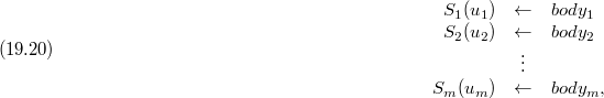
where relations of schema  do not occur in heads of rules, the same relation may appear in more than one rule head, furthermore there exists an ordering
  of the rules such that the relation of the head of rule
  does not occur in the head of any rule
  if
if  .
.
The computation of the result of nr-datalog  program (19.20) applied to instance
  over schema
  can be done in the same way as the evaluation of non-recursive datalog program (19.15), with the difference that the individual nr-datalog
  rules should be interpreted according to (19.19).
Example 19.5 Nr-datalog  program. Let us assume that all films that are included in relation Film have only one director. (It is not always true in real life!) The nr-datalog
  rule
rule

expresses query 19.6. Query 19.7 is realised by the nr-datalog  program

One has to be careful in writing nr-datalog  programs. If the first two rules of program (19.22) were to be merged like in Example 19.4

then (19.23) answers the following query (assuming that all films have unique director)
-
19.9 List all those films whose every actor played in each film of Fellini,
instead of query 19.7.
It is easy to see that every satisfiable nr-datalog  program that contains equality atoms can be replaced by one without equalities. Furthermore the following proposition is true, as well.
Claim 19.10 The satisfiable (full) relational algebra and the nr-datalog  programs with single output relation are equivalent query languages.
Query 19.8 cannot be formulated using the query languages introduced so far. Some a priori information would be needed about how long a chain-of-actors could be formed starting with a given actor/actress. Let us assume that the maximum length of a chain-of-actors starting from “Marcello Mastroianni” is 117. (It would be interesting to know the real value!) Then, the following non-recursive datalog program gives the answer.
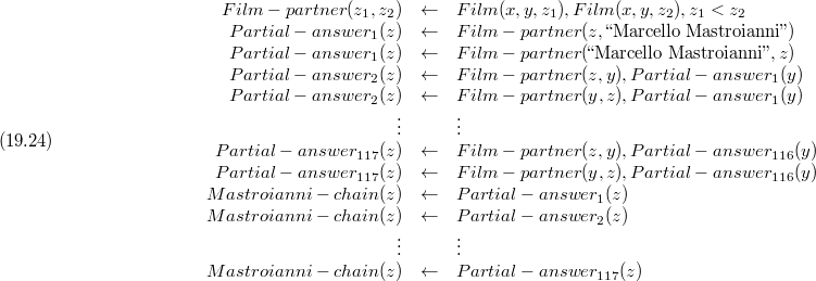
Footnote. Arbitrary comparison atoms can be used, as well, similarly to equality atoms. Here  makes it sure that all pairs occur at most once in the list.
It is much easier to express query 19.8 using recursion. In fact, the transitive closure of the graph Film-partner needs to be calculated. For the sake of simplicity the definition of Film-partner is changed a little (thus approximately doubling the storage requirement).

The datalog program (19.25) is recursive, since the definition of relation Chain-partner uses the relation itself. Let us suppose for a moment that this is meaningful, then query 19.8 is answered by rule

Definition 19.11 The expression

is a datalog rule, if  , the
, the  's are relation names, the
  's are free tuples of appropriate length. Every variable of
  has to occur in one of
  , as well. The head of the rule is
  , the body of the rule is
  . A datalog program is a finite collection of rules of type (19.27). Let
  be a datalog program. The relation
  occurring in
  is extensional if it occurs in only rule bodies, and it is intensional if it occurs in the head of some rule.
If  is a valuation of the variables of rule (19.27), then
  is a realisation of rule (19.27). The extensional (database) schema of
  consists of the extensional relations of
  , in notation
  . The intensional schema of
  , in notation
  is defined similarly as consisting of the intensional relations of
  . Let
. Let  . The semantics of datalog program
  is a mapping from the set of instances over
  to the set of instances over
  . This can be defined proof theoretically, model theoretically or as a fixpoint of some operator. This latter one is equivalent with the first two, so to save space only the fixpoint theoretical definition is discussed.
There are no negative literals used in Definition 19.11. The main reason of this is that recursion and negation together may be meaningless, or contradictory. Nevertheless, sometimes negative atoms might be necessary. In those cases the semantics of the program will be defined specially.
Let  be a datalog program,
  be an instance over
  . Fact
  , that is a tuple consisting of constants is an immediate consequence of
  and
and  , if either
  for some relation
  , or
, or  is a realisation of a rule in
  and each
  is in
is in  . The immediate consequence operator
  is a mapping from the set of instances over
  to itself.
  consists of all immediate consequences of
  and
and  .
.
Claim 19.12 The immediate consequence operator  is monotone.
Proof. Let  and
and  be instances over
  , such that
  . Let
. Let  be a fact of
  . If
. If  for some relation
  , then
  is implied by
  . on the other hand, if
  is a realisation of a rule in
  and each
  is in
is in  , then
  also holds.
The definition of  implies that
  . Using Proposition 19.12 it follows that

Theorem 19.13 For every instance  over schema
  there exists a unique minimal instance
  that is a fixpoint of
  , i.e.
  .
.
Proof. Let  denote the consecutive application of operator
 -times, and let

By the monotonicity of  and (19.29) we have

that is  is a fixpoint. It is easy to see that every fixpoint that contains
  , also contains
  for all
  , that is it contains
  , as well.
Definition 19.14 The result of datalog program  on instance
  over
over  is the unique minimal fixpoint of
  containing
  , in notation
  .
.
It can be seen, see Exercise 19.1-6, that the chain in (19.28) is finite, that is there exists an  , such that
  . The naive evaluation of the result of the datalog program is based on this observation.
Naiv-Datalog(
)
12
WHILE3
DO4
RETURN
Procedure Naiv-Datalog is not optimal, of course, since every fact that becomes included in  is calculated again and again at every further execution of the
 wHILE loop.
The idea of Semi-Naive-Datalog is that it tries to use only recently calculated new facts in the wHILE loop, as much as it is possible, thus avoiding recomputation of known facts. Consider datalog program  with
with  , and
, and  . For a rule

of  where
where  and
and  , the following rules are constructed for
  and
and 

Relation  denotes the change of
  in iteration
  . The union of rules corresponding to
  in layer
  is denoted by
  , that is rules of form (19.32) for
  ,
,  . Assume that the list of
  relations occurring in rules defining the
  relation
  is
is  . Let
. Let

denote the set of facts (tuples) obtained by applying rules (19.32) to input instance  and to
  relations
  . The input instance
  is the actual value of the
  relations of
  .
.
Semi-Naive-Datalog(
)
1those rules of
whose body does not contain
relation 2
FOR3
DO4
5
6
REPEAT7FOR8

are the
relations of the rules defining
. 9
DO10
11
12
UNTILfor all
13
FOR14
DO15
RETURN
Theorem 19.15 Procedure Semi-Naive-Datalog correctly computes the result of program  on instance
  .
.
Proof. We will show by induction on  that after execution of the loop of lines 6–12
  times the value of
  is
is  , while
  is equal to
  for arbitrary
  .
.  is the result obtained for
  starting from
  and applying the immediate consequence operator
 -times.
For  , line 4 calculates exactly
  for all
  . In order to prove the induction step, one only needs to see that
  is exactly equal to
  , since in lines 9–10 procedure
 Semi-Naive-Datalog constructs  -t and
  using that. The value of
  is
is  , by the induction hypothesis. Additional new tuples are obtained only if that for some
  relation defining
  such tuples are considered that are constructed at the last application of
  , and these are in relations
  , also by the induction hypothesis.
The halting condition of line 12 means exactly that all relations  are unchanged during the application of the immediate consequence operator
  , thus the algorithm has found its minimal fixpoint. This latter one is exactly the result of datalog program
  on input instance
  according to Definition 19.14.
Procedure Semi-Naive-Datalog eliminates a large amount of unnecessary calculations, nevertheless it is not optimal on some datalog programs (Exercise 19.1-7). However, analysis of the datalog program and computation based on that can save most of the unnecessary calculations.
Definition 19.16 Let  be a datalog program. The precedence graph of
  is the directed graph
  defined as follows. Its vertex set consists of the relations of
  , and
, and  is an arc for
  if there exists a rule in
  whose head is
  and whose body contains
  .
.  is recursive, if
  contains a directed cycle. Relations
  and
and  are mutually recursive if the belong to the same strongly connected component of
  .
.
Being mutually recursive is an equivalence relation on the set of relations  . The main idea of procedure
 Improved-Semi-Naive-Datalog is that for a relation  only those relations have to be computed “simultaneously” with
  that are in its equivalence class, all other relations defining
  can be calculated “in advance” and can be considered as
  relations.
Improved-Semi-Naive-Datalog(
)
1 Determine the equivalence classes ofunder mutual recursivity. 2 List the equivalence classes
according to a topological order of
. 3
There exists no directed path from
to
in
for all
. 4
FOR
TO5
DOUseSemi-Naive-Datalogto compute relations oftaking relations of
as
relations for
.
Lines 1–2 can be executed in time  using depth first search, where
  and
and  denote the number of vertices and edges of graph
  , respectively. Proof of correctness of the procedure is left to the Reader (Exercise 19.1-8).
In the present section we return to conjunctive queries. The costliest task in computing result of a query is to generate the natural join of relations. In particular, if there are no indexes available on the common attributes, hence only procedure Full-Tuplewise-Join is applicable.
Full-Tuplewise-Join(
)
12
FORall3
DOFORall4
DOIFand
can be joined 5
THEN6
RETURN
It is clear that the running time of Full-Tuplewise-Join is  . Thus, it is important that in what order is a query executed, since during computation natural joins of relations of various sizes must be calculated. In case of tableau queries the Homomorphism Theorem gives a possibility of a query rewriting that uses less joins than the original.
Let  be queries over schema
  .
.  contains
  , in notation
  , if for all instances
  over schema
 holds.
  according to Definition 19.1 iff
  and
and  . A generalisation of valuations will be needed. Substitution is a mapping from the set of variables to the union of sets of variables and sets of constants that is extended to constants as identity. Extension of substitution to free tuples and tableaux can be defined naturally.
Definition 19.17 Let  and
and  be two tableau queries overs schema
  . Substitution
  is a homomorphism from
  to
to  , if
, if  and
and  .
.
Theorem 19.18 (Homomorphism Theorem) Let  and
and  be two tableau queries overs schema
  .
.  if and only if, there exists a homomorphism from
  to
to  .
.
Proof. Assume first, that  is a homomorphism from
  to
to  , and let
  be an instance over schema
  . Let
. Let  . This holds exactly if there exists a valuation
  that maps tableau
  into
into  and
and  . It is easy to see that
  maps tableau
  into
into  and
and  , that is
  . Hence,
  , which in turn is equivalent with
  .
.
On the other hand, let us assume that  . The idea of the proof is that both,
  and
and  are applied to the “instance”
  . The output of
  is free tuple
  , hence the output of
  also contains
  , that is there exists a
  embedding of
  into
into  that maps
  to
to  . To formalise this argument the instance
  isomorphic to
  is constructed.
Let  be the set of variables occurring in
  . For all
  let
let  be constant that differs from all constants appearing in
  or
or  , furthermore
  . Let
. Let  be the valuation that maps
  to
to  , furthermore let
  .
.  is a bijection from
  to
to  and there are no constants of
  appearing in
  , hence
  well defined on the constants occurring in
  .
.
It is clear that  , thus using
 is obtained. That is, there exists a valuation
  that embeds tableau
  into
into  , such that
  . It is not hard to see that
  is a homomorphism from
  to
to  .
.
According to Theorem 19.6 tableau queries and satisfiable relational algebra (without subtraction) are equivalent. The proof shows that the relational algebra expression equivalent with a tableau query is of form  , where
  is the number of rows of the tableau. It implies that if the number of joins is to be minimised, then the number of rows of an equivalent tableau must be minimised.
The tableau query  is minimal, if there exists no tableau query
  that is equivalent with
  and
and  , that is
  has fewer rows. It may be surprising, but it is true, that a minimal tableau query equivalent with
  can be obtained by simply dropping some rows from
  .
.
Theorem 19.19 Let  be a tableau query. There exists a subset
  of
of  , such that query
  is minimal and equivalent with
  .
.
Proof. Let  be a minimal query equivalent with
  . According to the Homomorphism Theorem there exist homomorphisms
  from
from  to
to  , and
, and  from
from  to
to  . Let
. Let  . It is easy to check that
  and
and  . But
. But  is minimal, hence
  is minimal, as well.
Example 19.6 Application of tableau minimisation Consider the relational algebra expression

over the schema  of attribute set
  . The tableau query corresponding to
  is the following tableau
  :
:
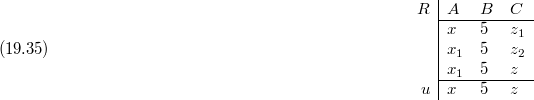
Such a homomorphism is sought that maps some rows of  to some other rows of
  , thus sort of “folding” the tableau. The first row cannot be eliminated, since the homomorphism is an identity on free tuple
  , thus
  must be mapped to itself. The situation is similar with the third row, as the image of
  is itself under any homomorphism. However the second row can be eliminated by mapping
  to
to  and
and  to
to  , respectively. Thus, the minimal tableau equivalent with
  consists of the first and third rows of
  . Transforming back to relational algebra expression,

is obtained. Query (19.36) contains one less join operator than query (19.34).
The next theorem states that the question of tableau containment and equivalence is NP-complete, hence tableau minimisation is an NP-hard problem.
Theorem 19.20 For given tableau queries  and
and  the following decision problems are NP-complete:
-
19.10
 ?
? -
19.11
 ?
? -
19.12 Assume that
 is obtained from
  by removing some free tuples. Is it true then that
  ?
?
Proof. The Exact-Cover problem will be reduced to the various tableau problems. The input of Exact-Cover problem is a finite set  , and a collection of its subsets
  . It has to be determined whether there exists
  , such that subsets in
  cover
cover  exactly (that is, for all
  there exists exactly one
  such that
  ).
). Exact-Cover is known to be an NP-complete problem.
Let  be an input of
 Exact-Cover. A construction is sketched that produces a pair  of tableau queries to
  in polynomial time. This construction can be used to prove the various NP-completeness results.
Let the schema  consist of the pairwise distinct attributes
  .
.  and
and  are tableau queries over schema
  such that the summary row of both of them is free tuple
  , where
  are pairwise distinct variables.
Let  be another set of pairwise distinct variables. Tableau
  consists of
  rows, for each element of
  corresponds one.
  stands in column of attribute
  in the row of
  , while
  stands in column of attribute
  for all such
  that
that  holds. In other positions of tableau
  pairwise distinct new variables stand.
Similarly,  consists of
  rows, one corresponding to each element of
  .
.  stands in column of attribute
  in the row of
  for all such
  that
that  , furthermore
  stands in the column of attribute
  , for all
  . In other positions of tableau
  pairwise distinct new variables stand.
The NP-completeness of problem 19.10 follows from that  has an exact cover using sets of
  if and only if
  holds. The proof, and the proof of the NP-completeness of problems 19.11 and 19.12 are left to the Reader (Exercise 19.1-9).
Exercises
19.1-1 Prove Proposition 19.4, that is every rule based query  is monotone and satisfiable. Hint. For the proof of satisfiability let
  be the set of constants occurring in query
  , and let
  be another constant. For every relation schema
  in rule (19.3) construct all tuples
  , where
  , and
, and  is the arity of
  . Let
. Let  be the instance obtained so. Prove that
  is nonempty.
19.1-2 Give a relational schema  and a relational algebra query
  over schema
  , whose result is empty to arbitrary instance over
  .
.
19.1-3 Prove that the languages of rule based queries and tableau queries are equivalent.
19.1-4 Prove that every rule based query  with equality atoms is either equivalent with the empty query
  , or there exists a rule based query
  without equality atoms such that
  . Give a polynomial time algorithm that determines for a rule based query
  with equality atoms whether
  holds, and if not, then constructs a rule based query
  without equality atoms, such that
  .
.
19.1-5 Prove Theorem 19.8 by generalising the proof idea of Theorem 19.6.
19.1-6 Let  be a datalog program,
  be an instance over
  ,
,  be the (finite) set of constants occurring in
  and
and  . Let
. Let  be the following instance over
  :
:
-
For every relation
 of
of  the fact
  is in
is in  iff it is in
  , furthermore
 -
for every relation
 of
of  every
every  fact constructed from constants of
  is in
is in  .
.
Prove that

19.1-7 Give an example of an input, that is a datalog program  and instance
  over
over  , such that the same tuple is produced by distinct runs of the loop of
 Semi-Naive-Datalog
19.1-8 Prove that procedure Improved-Semi-Naive-Datalog stops in finite time for all inputs, and gives correct result. Give an example of an input on which Improved-Semi-Naive-Datalog calculates less number of rows multiple times than Semi-Naive-Datalog.
-
Prove that for tableau queries
 and
and  of the proof of Theorem 19.20 there exists a homomorphism from
  to
to  if and only if the
 Exact-Coverproblem has solution.
 -
Prove that the decision problems 19.11 and 19.12 are NP-complete.
A database system architecture has three main levels:
-
physical layer;
-
logical layer;
-
outer (user) layer.
The goal of the separation of levels is to reach data independence and the convenience of users. The three views on Figure 19.2 show possible user interfaces: multirelational, universal relation and graphical interface.
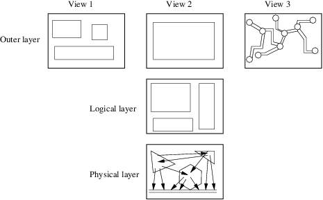
The physical layer consists of the actually stored data files and the dense and sparse indices built over them.
The separation of the logical layer from the physical layer makes it possible for the user to concentrate on the logical dependencies of the data, which approximates the image of the reality to be modelled better. The logical layer consists of the database schema description together with the various integrity constraints, dependencies. This the layer where the database administrators work with the system. The connection between the physical layer and the logical layer is maintained by the database engine.
The goal of the separation of the logical layer and the outer layer is that the endusers can see the database according to their (narrow) needs and requirements. For example, a very simple view of the outer layer of a bank database could be the automatic teller machine, or a much more complex view could be the credit history of a client for loan approval.
The question is that how can the views of different layers be given. If a query given by relational algebra expression is considered as a formula that will be applied to relational instances, then the view is obtained. Datalog rules show the difference between views and relations, well. The relations defined by rules are called intensional, because these are the relations that do not have to exist on external storage devices, that is to exist extensionally, in contrast to the extensional relations.
Definition 19.21 The  expression given in some query language
  over schema
  is called a view.
Similarly to intensional relations, views can be used in definition of queries or other views, as well.
Example 19.7 SQL view. Views in database manipulation language SQL can be given in the following way. Suppose that the only interesting data for us from schema CinePest is where and when are Kurosawa's film shown. The view KurosawaTimes is given by the SQL command
KurosawaTimes
1CREATEVIEWKurosawaTimesAS2SELECTTheater, Time 3FROMFilm, Show 4WHEREFilm.Title=Show.TitleANDFilm.Director="Akira Kurosawa"
Written in relational algebra is as follows.

Finally, the same by datalog rule is:

Line 2 of KurosawaTimes marks the selection operator used, line 3 marks that which two relations are to be joined, finally the condition of line 4 shows that it is a natural join, not a direct product.
Having defined view  , it can be used in further queries or view definitions like any other (extensional) relation.
-
Automatic data hiding: Such data that is not part of the view used, is not shown to the user, thus the user cannot read or modify them without having proper access rights to them. So by providing access to the database through views, a simple, but effective security mechanism is created.
-
Views provide simple “macro capabilities”. Using the view KurosawaTimes defined in Example 19.7 it is easy to find those theatres where Kurosawa films are shown in the morning:
Of course the user could include the definition of KurosawaTimes in the code directly, however convenience considerations are first here, in close similarity with macros.
-
Views make it possible that the same data could be seen in different ways by different users at the same time.
-
Views provide logical data independence. The essence of logical data independence is that users and their programs are protected from the structural changes of the database schema. It can be achieved by defining the relations of the schema before the structural change as views in the new schema.
-
Views make controlled data input possible. The
wITH CHECK OPTIONclause of commandcREATE VIEWis to do this in SQL.

Some view could be used in several different queries. It could be useful in these cases that if the tuples of the relation(s) defined by the view need not be calculated again and again, but the output of the query defining the view is stored, and only read in at further uses. Such stored output is called a materialised view.
Exercises
19.2-1 Consider the following schema:
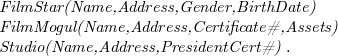
Relation FilmMogul contains data of the big people in film business (studio presidents, producers, etc.). The attribute names speak for themselves, Certificate# is the number of the certificate of the filmmogul, PresidentCert#) is the certificate number of the president of the studio. Give the definitions of the following views using datalog rules, relational algebra expressions, furthermore SQL:
-
RichMogul: Lists the names, addresses,certificate numbers and assets of those filmmoguls, whose asset value is over 1 million dollars.
-
StudioPresident: Lists the names, addresses and certificate numbers of those filmmoguls, who are studio presidents, as well.
-
MogulStar: Lists the names, addresses,certificate numbers and assets of those people who are filmstars and filmmoguls at the same time.
19.2-2 Give the definitions of the following views over schema CinePest using datalog rules, relational algebra expressions, furthermore SQL:
-
Marilyn(Title): Lists the titles of Marilyn Monroe's films.
-
CorvinInfo(Title,Time,Phone): List the titles and show times of films shown in theatre Corvin, together with the phone number of the theatre.
Answering queries using views, in other words query rewriting using views has become a problem attracting much attention and interest recently. The reason is its applicability in a wide range of data manipulation problems: query optimisation, providing physical data independence, data and information integration, furthermore planning data warehouses.
The problem is the following. Assume that query  is given over schema
  , together with views
  . Can one answer
  using only the results of views
  ? Or, which is the largest set of tuples that can be determined knowing the views? If the views and the relations of the base schema can be accessed both, what is the cheapest way to compute the result of
  ?
?
Before query rewriting algorithms are studied in detail, some motivating examples of applications are given. The following university database is used throughout this section.

The schemata of the individual relations are as follows:
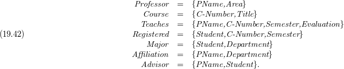
It is supposed that professors, students and departments are uniquely identified by their names. Tuples of relation Registered show that which student took which course in what semester, while Major shows which department a student choose in majoring (for the sake of convenience it is assumed that one department has one subject as possible major).
If the computation necessary to answer a query was performed in advance and the results are stored in some materialised view, then it can be used to speed up the query answering.
Consider the query that looks for pairs (Student,Title), where the student registered for the given Ph.D.-level course, the course is taught by a professor of the Database area (the C-number of graduate courses is at least 400, and the Ph.D.-level courses are those with C-number at least 500).

Suppose that the following materialised view is available that contains the registration data of graduate courses.

View Graduate can be used to answer query (19.43).

It will be faster to compute (19.45) than to compute (19.43), because the natural join of relations Registered and Course has already be done by view Graduate, furthermore it shelled off the undergraduate courses (that make up for the bulk of registration data at most universities). It worth noting that view Graduate could be used event hough syntactically did not agree with any part of query (19.43).
On the other hand, it may happen that the the original query can be answered faster. If relations Registered and Course have an index on attribute C-Number, but there exists no index built for Graduate, then it could be faster to answer query (19.43) directly from the database relations. Thus, the real challenge is not only that to decide about a materialised view whether it could be used to answer some query logically, but a thorough cost analysis must be done when is it worth using the existing views.
One of the principles underlying modern database systems is the separation between the logical view of data and the physical view of data. With the exception of horizontal or vertical partitioning of relations into multiple files, relational database systems are still largely based on a one-to-one correspondence between relations in the schema and the files in which they are stored. In object-oriented systems, maintaining the separation is necessary because the logical schema contains significant redundancy, and does not correspond to a good physical layout. Maintaining physical data independence becomes more crucial in applications where the logical model is introduced as an intermediate level after the physical representation has already been determined. This is common in storage of XML data in relational databases, and in data integration. In fact, the Stored System stores XML documents in a relational database, and uses views to describe the mapping from XML into relations in the database.
To maintain physical data independence, a widely accepted method is to use views over the logical schema as mechanism for describing the physical storage of data. In particular, Tsatalos, Solomon and Ioannidis use GMAPs (Generalised Multi-level Access Paths) to describe data storage.
A GMAP describes the physical organisation and the indexes of the storage structure. The first clause of the GMAP (aS) describes the actual data structure used to store a set of tuples (e.g., a  -tree, hash index, etc.) The remaining clauses describe the content of the structure, much like a view definition. The
 gIVEN and sELECT clauses describe the available attributes, where the gIVEN clause describes the attributes on which the structure is indexed. The definition of the view, given in the wHERE clause uses infix notation over the conceptual model.
In the example shown in Figure 19.3 the GMAP G1 stores a set of pairs containing students and the departments in which they major, and these pairs are indexed by a  -tree on attribute Student.name. The GMAP G2 stores an index from names of students to the numbers of courses in which they are registered. The GMAP G3 stores an index from course numbers to departments whose majors are enrolled in the course.
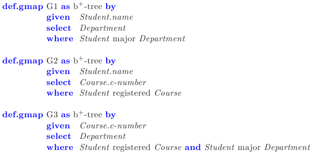
Given that the data is stored in structures described by the GMAPs, the question that arises is how to use these structures to answer queries. Since the logical content of the GMAPs are described by views, answering a query amounts to finding a way of rewriting the query using these views. If there are multiple ways of answering the query using the views, we would like to find the cheapest one. Note that in contrast to the query optimisation context, we must use the views to answer the given query, because all the data is stored in the GMAPs.
Consider the following query, which asks for names of students registered for Ph.D.-level courses and the departments in which these students are majoring.

The query can be answered in two ways. First, since Student.name uniquely identifies a student, we can take the join of G! and G2, and then apply selection operator  , finally a projection eliminates the unnecessary attributes. The other execution plan could be to join G3 with G2 and select
  . In fact, this solution may even be more efficient because G3 has an index on the course number and therefore the intermediate joins may be much smaller.
A data integration system (also known as mediator system) provides a uniform query interface to a multitude of autonomous heterogeneous data sources. Prime examples of data integration applications include enterprise integration, querying multiple sources on the World-Wide Web, and integration of data from distributed scientific experiments.
To provide a uniform interface, a data integration system exposes to the user a mediated schema. A mediated schema is a set of virtual relations, in the sense that they are not stored anywhere. The mediated schema is designed manually for a particular data integration application. To be able to answer queries, the system must also contain a set of source descriptions. A description of a data source specifies the contents of the source, the attributes that can be found in the source, and the (integrity) constraints on the content of the source. A widely adopted approach for specifying source descriptions is to describe the contents of a data source as a view over the mediated schema. This approach facilitates the addition of new data sources and the specification of constraints on the contents of sources.
In order to answer a query, a data integration system needs to translate a query formulated on the mediated schema into one that refers directly to the schemata of the data sources. Since the contents of the data sources are described as views, the translation problem amounts finding a way to answer a query using a set of views.
Consider as an example the case where the mediated schema exposed to the user is schema University, except that the relations Teaches and Course have an additional attribute identifying the university at which the course is being taught:

Suppose we have the following two data sources. The first source provides a listing of all the courses entitled "Database Systems" taught anywhere and their instructors. This source can be described by the following view definition:

The second source lists Ph.D.-level courses being taught at The Ohio State University (OSU), and is described by the following view definition:

If we were to ask the data integration system who teaches courses titled "Database Systems" at OSU, it would be able to answer the query by applying a selection on the source DB-courses:

On the other hand, suppose we ask for all the graduate-level courses (not just in databases) being offered at OSU. Given that only these two sources are available, the data integration system cannot find all tuples in the answer to the query. Instead, the system can attempt to find the maximal set of tuples in the answer available from the sources. In particular, the system can obtain graduate database courses at OSU from the DB-course source, and the Ph.D.-level courses at OSU from the OSUPhD source. Hence, the following non-recursive datalog program gives the maximal set of answers that can be obtained from the two sources:

Note that courses that are not PH.D.-level courses or database courses will not be returned as answers. Whereas in the contexts of query optimisation and maintaining physical data independence the focus is on finding a query expression that is equivalent with the original query, here finding a query expression that provides the maximal answers from the views is attempted.
If the database is accessed via client-server architecture, the data cached at the client can be semantically modelled as results of certain queries, rather than at the physical level as a set of data pages or tuples. Hence, deciding which data needs to be shipped from the server in order to answer a given query requires an analysis of which parts of the query can be answered by the cached views.
In this section the theoretical complexity of query rewriting is studied. Mostly conjunctive queries are considered. Minimal, and complete rewriting will be distinguished. It will be shown that if the query is conjunctive, furthermore the materialised views are also given as results of conjunctive queries, then the rewriting problem is NP-complete, assuming that neither the query nor the view definitions contain comparison atoms. Conjunctive queries will be considered in rule-based form for the sake of convenience.
Assume that query  is given over schema
  .
.
Definition 19.22 The conjunctive query  is a rewriting of query
  using views
  , if
, if
-
 and
and  are equivalent, and
 -
 contains one or more literals from
  .
.
 is said to be locally minimal if no literal can be removed from
  without violating the equivalence. The rewriting is globally minimal, if there exists no rewriting using a smaller number of literals. (The comparison atoms
  are not counted in the number of literals.)
Example 19.8 Query rewriting. Consider the following query  and view
  .
.

 can be rewritten using
  :
:

View  replaces the first two literals of query
  . Note that the view certainly satisfies the third literal of the query, as well. However, it cannot be removed from the rewriting, since variable
  does not occur in the head of
  , thus if literal
  were to be removed, too, then the natural join of
  and
and  would not be enforced anymore.
Since in some of the applications the database relations are inaccessible, only the views can be accessed, for example in case of data integration or data warehouses, the concept of complete rewriting is introduced.
Definition 19.23 A rewriting  of query
  using views
 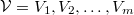 is called a complete rewriting, if
  contains only literals of
  and comparison atoms.
Example 19.9 Complete rewriting. Assume that besides view  of Example 19.8 the following view is given, as well:

A complete rewriting of query  is:
is:

It is important to see that this rewriting cannot be obtained step-by-step, first using only  , then trying to incorporate
  , (or just in the opposite order) since relation
  of
of  does not occur in
  . Thus, in order to find the complete rewriting, use of the two view must be considered parallel, at the same time.
There is a close connection between finding a rewriting and the problem of query containment. This latter one was discussed for tableau queries in section 19.1.3. Homomorphism between tableau queries can be defined for rule based queries, as well. The only difference is that it is not required in this section that a homomorphism maps the head of one rule to the head of the other. (The head of a rule corresponds to the summary row of a tableau.) According to Theorem 19.20 it is NP-complete to decide whether conjunctive query  contains another conjunctive query
  . This remains true in the case when
  may contain comparison atoms, as well. However, if both,
  and
and  may contain comparison atoms, then the existence of a homomorphism from
  to
to  is only a sufficient but not necessary condition for the containment of queries, which is a
  -complete problem in that case. The discussion of this latter complexity class is beyond the scope of this chapter, thus it is omitted. The next proposition gives a necessary and sufficient condition whether there exists a rewriting of query
  using view
  .
.
Claim 19.24 Let  and
and  be conjunctive queries that may contain comparison atoms. There exists a a rewriting of query
  using view
  if and only if
  , that is the projection of
  to the empty attribute set contains that of
  .
.
Proof. Observe that 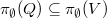 is equivalent with the following proposition: If the output of
  is empty for some instance, then the same holds for the output of
  , as well.
Assume first that there exists a rewriting, that is a rule equivalent with  that contains
  in its body. If
  is such an instance, that the result of
  is empty on it, then every rule that includes
  in its body results in empty set over
  , too.
In order to prove the other direction, assume that if the output of  is empty for some instance, then the same holds for the output of
  , as well. Let

Let  be a list of variables disjoint from variables of
  . Then the query
  defined by

satisfies  . It is clear that
  . On the other hand, if there exists a valuation of the variables of
  that satisfies the body of
  over some instance
  , then fixing it, for arbitrary valuation of variables in
  a tuple is obtained in the output of
  , whenever a tuple is obtained in the output of
  together with the previously fixed valuation of variables of
  .
.
As a corollary of Theorem 19.20 and Proposition 19.24 the following theorem is obtained.
Theorem 19.25 Let  be a conjunctive query that may contain comparison atoms, and let
  be a set of views. If the views in
  are given by conjunctive queries that do not contain comparison atoms, then it is NP-complete to decide whether there exists a rewriting of
  using
using  .
.
The proof of Theorem 19.25 is left for the Reader (Exercise 19.3-1).
The proof of Proposition 19.24 uses new variables. However, according to the next lemma, this is not necessary. Another important observation is that it is enough to consider a subset of database relations occurring in the original query when locally minimal rewriting is sought, new database relations need not be introduced.
Lemma 19.26 Let  be a conjunctive query that does not contain comparison atoms

furthermore let  be a set of views that do not contain comparison atoms either.
-
If
 is a locally minimal rewriting of
  using
using  , then the set of database literals in
  is isomorphic to a subset of database literals occurring in
  .
. -
If
is a rewriting of
 using the views, then there exists a rewriting
 such that
 , that is the rewriting does not introduce new variables.


The details of the proof of Lemma 19.26 are left for the Reader (Exercise 19.3-2). The next lemma is of fundamental importance: A minimal rewriting of  using
using  cannot increase the number of literals.
Lemma 19.27 Let  be conjunctive query,
  be set of views given by conjunctive queries, both without comparison atoms. If the body of
  contains
  literals and
  is a locally minimal rewriting of
  using
using  , then
  contains at most
  literals.
Proof. Replacing the view literals of  by their definitions query
  is obtained. Let
  be a homomorphism from the body of
  to
to  . The existence of
  follows from
  by the Homomorphism Theorem (Theorem 19.18). Each of the literals
  of the body of
  is mapped to at most one literal obtained from the expansion of view definitions. If
  contains more than
  view literals, then the expansion of some view literals in the body of
  is disjoint from the image of
  . These view literals can be removed from the body of
  without changing the equivalence.
Based on Lemma 19.27 the following theorem can be stated about complexity of minimal rewritings.
Theorem 19.28 Let  be conjunctive query,
  be set of views given by conjunctive queries, both without comparison atoms. Let the body of
  contain
  literals.
-
It is NP-complete to decide whether there exists a rewriting
 of
of  using
using  that uses at most
  literals.
 -
It is NP-complete to decide whether there exists a rewriting
 of
of  using
using  that uses at most
  database literals.
 -
It is NP-complete to decide whether there exists a complete rewriting of
 using
using  .
.
Proof. The first statement is proved, the proof of the other two is similar. According to Lemmas 19.27 and 19.26, only such rewritings need to be considered that have at most as many literals as the query itself, contain a subset of the literals of the query and do not introduce new variables. Such a rewriting and the homomorphisms proving the equivalence can be tested in polynomial time, hence the problem is in NP. In order to prove that it is NP-hard, Theorem 19.25 is used. For a given query  and view
  let
let  be the view, whose head is same as the head of
  , but whose body is the conjunction of the bodies of
  and
and  . It is easy to see that there exists a rewriting using
  with a single literal if and only if there exists a rewriting (with no restriction) using
  .
.
In this section only complete rewritings are studied. This does not mean real restriction, since if database relations are also to be used, then views mirroring the database relations one-to-one can be introduced. The concept of equivalent rewriting introduced in Definition 19.22 is appropriate if the goal of the rewriting is query optimisation or providing physical data independence. However, in the context of data integration on data warehouses equivalent rewritings cannot be sought, since all necessary data may not be available. Thus, the concept of maximally contained rewriting is introduced that depends on the query language used, in contrast to equivalent rewritings.
Definition 19.29 Let  be a query,
  be a set of views,
  be a query language.
  is a maximally contained rewriting of
  with respect to
  , if
, if
-
 is a query of language
  using only views from
  ,
, -
 contains
  ,
, -
if query
 satisfies
  , then
  .
.
Before discussing how can a traditional optimiser be modified in order to use materialised views instead of database relations, it is necessary to survey when can view be used to answer a given query. Essentially, view  can be used to answer query
  , if the intersection of the sets of database relations in the body of
  and in the body of
  is non-empty, furthermore some of the attributes are selected by
  are also selected by
  . Besides this, in case of equivalent rewriting, if
  contains comparison atoms for such attributes that are also occurring in
  , then the view must apply logically equivalent, or weaker condition, than the query. If logically stronger condition is applied in the view, then it can be part of a (maximally) contained rewriting. This can be shown best via an example. Consider the query
  over schema University that list those professor, student, semester triplets, where the advisor of the student is the professor and in the given semester the student registered for some course taught by the professor.
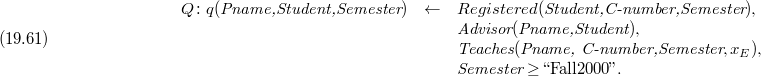
View  below can be used to answer
  , since it uses the same join condition for relations Registered and Teaches as
  , as it is shown by variables of the same name. Furthermore,
  selects attributes Student, PName, Semester, that are necessary in order to properly join with relation Advisor, and for select clause of the query. Finally, the predicate
  is weaker than the predicate
  of the query.

The following four views illustrate how minor modifications to  change the usability in answering the query.


View  is similar to
  , except that it does not select the attribute PName from relation Teaches, which is needed for the join with the relation Adviser and for the selection of the query. Hence, to use
  in the rewriting, it has to be joined with relation Teaches again. Still, if the join of relations Registered and Teaches is very selective, then employing
  may actually result in a more efficient query execution plan.
In view  the join of relations Registered and Teaches is over only attribute C-number, the equality of variables Semester and
  is not required. Since attribute
  is not selected by
  , the join predicate cannot be applied in the rewriting, and therefore there is little gain by using
  .
.
View  considers only the professors who have at least one area of research. Hence, the view applies an additional condition that does not exists in the query, and cannot be used in an equivalent rewriting unless union and negation are allowed in the rewriting language. However, if there is an integrity constraint stating that every professor has at least one area of research, then an optimiser should be able to realise that
  is usable.
Finally, view  applies a stronger predicate than the query, and is therefore usable for a contained rewriting, but not for an equivalent rewriting of the query.
System-R style optimisation
Before discussing the changes to traditional optimisation, first the principles underlying the System-R style optimiser is recalled briefly. System-R takes a bottom-up approach to building query execution plans. In the first phase, it concentrates of plans of size 1, i.e., chooses the best access paths to every table mentioned in the query. In phase  , the algorithm considers plans of size
  , by combining plans obtained in the previous phases (sizes of
  and
and  ). The algorithm terminates after constructing plans that cover all the relations in the query. The efficiency of System-R stems from the fact that it partitions query execution plans into equivalence classes, and only considers a single execution plan for every equivalence class. Two plans are in the same equivalence class if they
-
cover the same set of relations in the query (and therefore are also of the same size), and
-
produce the answer in the same interesting order.
In our context, the query optimiser builds query execution plans by accessing a set of views, rather than a set of database relations. Hence, in addition to the meta-data that the query optimiser has about the materialised views (e.g., statistics, indexes) the optimiser is also given as input the query expressions defining the views. Th additional issues that the optimiser needs to consider in the presence of materialised views are as follows.
A. In the first iteration the algorithm needs to decide which views are relevant to the query according to the conditions illustrated above. The corresponding step is trivial in a traditional optimiser: a relation is relevant to the query if it is in the body of the query expression.
B. Since the query execution plans involve joins over views, rather than joins over database relations, plans can no longer be neatly partitioned into equivalence classes which can be explored in increasing size. This observation implies several changes to the traditional algorithm:
1. Termination testing: the algorithm needs to distinguish partial query execution plans of the query from complete query execution plans. The enumeration of the possible join orders terminates when there are no more unexplored partial plans. In contrast, in the traditional setting the algorithm terminates after considering the equivalence classes that include all the relations of the query.
2. Termination testing: the algorithm needs to distinguish partial query execution plans of the query from complete query execution plans. The enumeration of the possible join orders terminates when there are no more unexplored partial plans. In contrast, in the traditional setting the algorithm terminates after considering the equivalence classes that include all the relations of the query.
(a) is cheaper than  , and
, and
(b) has greater or equal contribution to the query than  . Informally, a plan
  contributes more to the query than plan
  if it covers more of the relations in the query and selects more of the necessary attributes.
3. Combining partial plans: in the traditional setting, when two partial plans are combined, the join predicates that involve both plans are explicit in the query, and the enumeration algorithm need only consider the most efficient way to apply these predicates. However, in our case, it may not be obvious a priori which join predicate will yield a correct rewriting of the query, since views are joined rather than database relations directly. Hence, the enumeration algorithm needs to consider several alternative join predicates. Fortunately, in practice, the number of join predicates that need to be considered can be significantly pruned using meta-data about the schema. For example, there is no point in trying to join a string attribute with a numeric one. Furthermore, in some cases knowledge of integrity constraints and the structure of the query can be used to reduce the number of join predicates to be considered. Finally, after considering all the possible join predicates, the optimiser also needs to check whether the resulting plan is still a partial solution to the query.
The following table summarises the comparison of the traditional optimiser versus one that exploits materialised views.
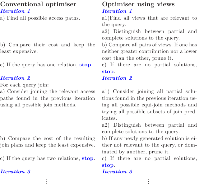
Another method of equivalent rewriting is using transformation rules. The common theme in the works of that area is that replacing some part of the query with a view is considered as another transformation available to the optimiser. These methods are not discussed in detail here.
The query optimisers discussed above were designed to handle cases where the number of views is relatively small (i.e., comparable to the size of the database schema), and cases where equivalent rewriting is required. In contrast, the context of data integration requires consideration of large number of views, since each data source is being described by one or more views. In addition, the view definitions may contain many complex predicates, whose goal is to express fine-grained distinction between the contents of different data sources. Furthermore, in the context of data integration it is often assumed that the views are not complete, i.e., they may only contain a subset of the tuples satisfying their definition. In the foregoing, some algorithms for answering queries using views are described that were developed specifically for the context of data integration.
The goal of the Bucket Algorithm is to reformulate a user query that is posed on a mediated (virtual) schema into a query that refers directly to the available sources. Both the query and the sources are described by conjunctive queries that may include atoms of arithmetic comparison predicates. The set of comparison atoms of query  is denoted by
  .
.
Since the number of possible rewritings may be exponential in the size of the query, the main idea underlying the bucket algorithm is that the number of query rewritings that need to be considered can be drastically reduced if we first consider each subgoal – the relational atoms of the query – is considered in isolation, and determine which views may be relevant to each subgoal.
The algorithm proceeds as follows. First, a bucket is created for each subgoal in the query  that is not in
  , containing the views that are relevant to answering the particular subgoal. In the second step, all such conjunctive query rewritings are considered that include one conjunct (view) from each bucket. For each rewriting
  obtained it is checked that whether it is semantically correct, that is
  holds, or whether it can be made semantically correct by adding comparison atoms. Finally the remaining plans are minimised by pruning redundant subgoals. Algorithm
 Create-Bucket executes the first step described above. Its input is a set of source descriptions  and a conjunctive query
  in the form

Create-Bucket(
)
1FOR
TO2
DO3
FORall4

is of form
. 5
DOFOR
TO6
IF7
THENletbe a mapping defined on the variables of
as follows: 8
IFis the
variable of
and
9
THEN, where
is the
variable of
10
ELSEis a new variable that does not appear in
or
. 11

12
IF13
THENaddto
14
RETURNBucket
Procedure  is the extension of
 Satisfiable described in section 19.1.2 to the case when comparison atoms may occur besides equality atoms. The necessary change is only that for all variable  occurring in comparison atoms it must be checked whether all predicates involving
  are satisfiable simultaneously.
Create-Bucket running time is polynomial function of the sizes of  and
and  . Indeed, the kernel of the nested loops of lines 3 and 5 runs
  times. The commands of lines 6–13 require constant time, except for line 12. The condition of of command
 iF in line 12 can be checked in polynomial time.
In order to prove the correctness of procedure Create-Bucket, one should check under what condition is a view  put in
  . In line 6 it is checked whether relation
  appears as a subgoal in
  . If not, then obviously
  cannot give usable information for subgoal
  of
of  . If
. If  is a subgoal of
  , then in lines 9–10 a mapping is constructed that applied to the variables allows the correspondence between subgoals
  and
and  , in accordance with relations occurring in the heads of
  and
and  , respectively. Finally, in line 12 it is checked whether the comparison atoms contradict with the correspondence constructed.
In the second step, having constructed the buckets using Create-Bucket, the bucket algorithm finds a set of conjunctive query rewritings, each of them being a conjunctive query that includes one conjunct from every bucket. Each of these conjunctive query rewritings represents one way of obtaining part of the answer to  from the views. The result of the bucket algorithm is defined to be the union of the conjunctive query rewritings (since each of the rewritings may contribute different tuples). A given conjunctive query
  is a conjunctive query rewriting, if
-
 , or
, or -
 can be extended with comparison atoms, so that the previous property holds.
Example 19.10 Bucket algorithm. Consider the following query  that lists those articles
  that there exists another article
  of the same area such that
  and
and  mutually cites each other. There are three views (sources) available,
  .
.
In the first step, applying Create-Bucket, the following buckets are constructed.

In the second step the algorithm constructs a conjunctive query  from each element of the Cartesian product of the buckets, and checks whether
  is contained in
  . If yes, it is given to the answer.
In our case, it tries to match  with the other views, however no correct answer is obtained so. The reason is that
  does not appear in the head of
  , hence the join condition of
  – variables
  and
and  occur in relation sameArea, as well – cannot be applied. Then rewritings containing
  are considered, recognising that equating the variables in the head of
  a contained rewriting is obtained. Finally, the algorithm finds that combining
  and
and  rewriting is obtained, as well. This latter is redundant, as it is obtained by simple checking, that is
  can be pruned. Thus, the result of the bucket algorithm for query (19.68) is the following (actually equivalent) rewriting

The strength of the bucket algorithm is that it exploits the predicates in the query to prune significantly the number of candidate conjunctive rewritings that need to be considered. Checking whether a view should belong to a bucket can be done in time polynomial in the size of the query and view definition when the predicates involved are arithmetic comparisons. Hence, if the data sources (i.e., the views) are indeed distinguished by having different comparison predicates, then the resulting buckets will be relatively small.
The main disadvantage of the bucket algorithm is that the Cartesian product of the buckets may still be large. Furthermore, the second step of the algorithm needs to perform a query containment test for every candidate rewriting, which is NP-complete even when no comparison predicates are involved.
The Inverse-rules algorithm is a procedure that can be applied more generally than the Bucket algorithm. It finds a maximally contained rewriting for any query given by arbitrary recursive datalog program that does not contain negation, in polynomial time.
The first question is that for given datalog program  and set of conjunctive queries
  , whether there exists a datalog program
  equivalent with
  , whose edb relations are relations
  of
of  . Unfortunately, this is algorithmically undecidable. Surprisingly, the best, maximally contained rewriting can be constructed. In the case, when there exists a datalog program
  equivalent with
  , the algorithm finds that, since a maximally contained rewriting contains
  , as well. This seemingly contradicts to the fact that the existence of equivalent rewriting is algorithmically undecidable, however it is undecidable about the result of the inverse-rules algorithm, whether it is really equivalent to the original query.
Example 19.11 Equivalent rewriting. Consider the following datalog program  , where edb relations edge and
  contain the edges and vertices coloured black of a graph
  .
.

It is easy to check that  lists the endpoints of such paths (more precisely walks) of graph
  whose inner points are all black. Assume that only the following two views can be accessed.

 stores edges whose tail is black, while
  stores those, whose head is black. There exists an equivalent rewriting
  of datalog program
  that uses only views
  and
and  as edb relations:

However, if only  , or
, or  is accessible alone, then equivalent rewriting is not possible, since only such paths are obtainable whose starting, or respectively, ending vertex is black.
In order to describe the Inverse-rules Algorithm, it is necessary to introduce the Horn rule, which is a generalisation of datalog program, and datalog rule. If function symbols are also allowed in the free tuple  of rule (19.27) in Definition 19.11, besides variables and constants, then Horn rule is obtained. A logic program is a collection of Horn rules. In this sense a logic program without function symbols is a datalog program. The concepts of
  and
and  can be defined for logic programs in the same way as for datalog programs.
The Inverse-rules Algorithm consists of two steps. First, a logic program is constructed that may contain function symbols. However, these will not occur in recursive rules, thus in the second step they can be eliminated and the logic program can be transformed into a datalog program.
Definition 19.30 The inverse  of view
  given by

is the following collection of Horn rules. A rule corresponds to every subgoal  , whose body is the literal
  . The head of the rule is
  , where
  is obtained from
  by preserving variables appearing in the head of rule (19.74), while function symbol
  is written in place of every variable
  not appearing the head. Distinct function symbols correspond to distinct variables. The inverse of a set
  of views is the set
  , where distinct function symbols occur in the inverses of distinct rules.
The idea of the definition of inverses is that if a tuple  appears in a view
  , for some constants
  , then there is a valuation of every variable
  appearing in the head that makes the body of the rule true. This “unknown” valuation is denoted by the function symbol
  .
.
Example 19.12 Inverse of views. Let  be the following collection of views.

Then  consists of the following rules.
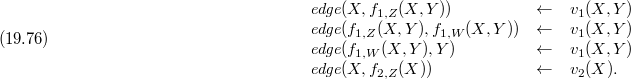
Now, the maximally contained rewriting of datalog program  using views
  can easily be constructed for given
  and
and  .
.
First, those rules are deleted from  that contain such edb relation that do not appear in the definition any view from
  . The rules of
  are added the datalog program
  obtained so, thus forming logic program
  . Note, that the remaining edb relations of
  are idb relations in logic program
  , since they appear in the heads of the rules of
  . The names of idb relations are arbitrary, so they can be renamed so that their names do not coincide with the names of edb relations of
  . However, this is not done in the following example, for the sake of better understanding.
Example 19.13 Logic program. Consider the following datalog program that calculates the transitive closure of relation edge.

Assume that only the following materialised view is accessible, that stores the endpoints of paths of length two. If only this view is usable, then the most that can be expected is listing the endpoints of paths of even length. Since the unique edb relation of datalog program  is edge, that also appears in the definition of
  , the logic program
  is obtained by adding the rules of
  to
to  .
.
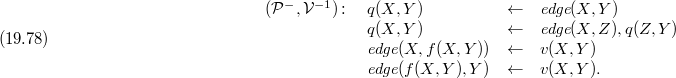
Let the instance of the edb relation edge of datalog program  be the graph
  shown on Figure 19.4.
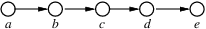
Then  introduces three new constants,
  és
és  . The idb relation edge of logic program
  is graph
  shown on Figure 19.5.
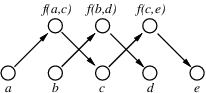
 computes the transitive closure of graph
  . Note that those pairs in th transitive closure that do not contain any of the new constants are exactly the endpoints of even paths of
  .
.
The result of logic program  in Example 19.13 can be calculated by procedure
  , for example. However, it is not true for logic programs in general, that the algorithm terminates. Indeed, consider the logic program

If the edb relation  contains the constant
  , then the output of the program is the infinite sequence
  . In contrary to this, the output of the logic program
  given by the Inverse-rules Algorithm is guaranteed to be finite, thus the computation terminates in finite time.
Theorem 19.31 For arbitrary datalog program  and set of conjunctive views
  , and for finite instances of the views, there exist a unique minimal fixpoint of the logic program
  , furthermore procedures
 Naiv-Datalog and Semi-Naive-Datalog give this minimal fixpoint as output.
The essence of the proof of Theorem 19.31 is that function symbols are only introduced by inverse rules, that are in turn not recursive, thus terms containing nested functions symbols are not produced. The details of the proof are left for the Reader (Exercise 19.3-3).
Even if started from the edb relations of a database, the output of a logic program may contain tuples that have function symbols. Thus, a filter is introduced that eliminates the unnecessary tuples. Let database  be the instance of the edb relations of datalog program
  .
.  denotes the set of those tuples from
  that do not contain function symbols. Let
  denote that program, which computes
  for a given instance
  . The proof of the following theorem, exceeds the limitations of the present chapter.
Theorem 19.32 For arbitrary datalog program  and set of conjunctive views
  , the logic program
  is a maximally contained rewriting of
  using
using  . Furthermore,
  can be constructed in polynomial time of the sizes of
  and
and  .
.
The meaning of Theorem 19.32 is that the simple procedure of adding the inverses of view definitions to a datalog program results in a logic program that uses the views as much as possible. It is easy to see that  can be constructed in polynomial time of the sizes of
  and
and  , since for every subgoal
  a unique inverse rule must be constructed.
In order to completely solve the rewriting problem however, a datalog program needs to be produced that is equivalent with the logic program  . The key to this is the observation that
  contains only finitely many function symbols, furthermore during a bottom-up evaluation like
 Naiv-Datalog and its versions, nested function symbols are not produced. With proper book keeping the appearance of function symbols can be kept track, without actually producing those tuples that contain them.
The transformation is done bottom-up like in procedure Naiv-Datalog. The function symbol  appearing in the idb relation of
  is replaced by the list of variables
  . At same time the name of the idb relation needs to be marked, to remember that the list
  belongs to function symbol
  . Thus, new “temporary” relation names are introduced. Consider the the rule

of the logic program (19.78) in Example 19.13. It is replaced by rule

Notation  means that the first argument of
  is the same as the first argument of
  , while the second and third arguments of
  together with function symbol
  give the second argument of
  . If a function symbol would become an argument of an idb relation of
  during the bottom-up evaluation of
  , then a new rule is added to the program with appropriately marked relation names.
Example 19.14 Transformation of logic program into datalog program. The logic program Example 19.13 is transformed to the following datalog program by the procedure sketched above. The different phases of the bottom-up execution of Naiv-Datalog are separated by lines.
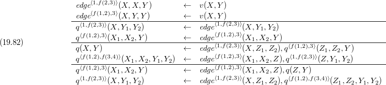
The datalog program obtained shows clearly that which arguments could involve function symbols in the original logic program. However, some rows containing function symbols never give tuples not containing function symbols during the evaluation of the output of the program.
Relation  is called significant, if in the precedence graph of Definition 19.16there exists oriented path from
  to the output relation of
  . If
. If  is not significant, then the tuples of
  are not needed to compute the output of the program, thus
  can be eliminated from the program.
Footnote. Here the definition of precedence graph needs to be extended for the edb relations of the datalog program, as well.
Example 19.15 Eliminating non-significant relations. There exists no directed path in the precedence graph of the datalog program obtained in Example 19.14, from relations  and
and  to the output relation
  of the program, thus they are not significant, i.e., they can be eliminated together with the rules that involve them. The following datalog program is obtained:
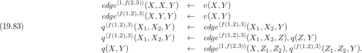
One more simplification step can be performed, which does not decrease the number of necessary derivations during computation of the output, however avoids redundant data copying. If  is such a relation in the datalog program that is defined by a single rule, which in turn contains a single relation in its body, then
  can be removed from the program and replaced by the relation of the body of the rule defining
  , having equated the variables accordingly.
Example 19.16 Avoiding unnecessary data copying. In Example 19.14 the relations  and
and  are defined by a single rule, respectively, furthermore these two rules both have a single relation in their bodies. Hence, program (19.83) can be simplified further.

The datalog program obtained in the two simplification steps above is denoted by  . It is clear that there exists a one-to-one correspondence between the bottom-up evaluations of
  and
and  . Since the function symbols in
  are kept track, it is sure that the output instance obtained is in fact the subset of tuples of the output of
  that do not contain function symbols.
Theorem 19.33 For arbitrary datalog program  that does not contain negations, and set of conjunctive views
  , the logic program
  is equivalent with the datalog program
  .
.
The main disadvantage of the Bucket Algorithm is that it considers each of the subgoals in isolation, therefore does not observe the most of the interactions between the subgoals of the views. Thus, the buckets may contain many unusable views, and the second phase of the algorithm may become very expensive.
The advantage of the Inverse-rules Algorithm is its conceptual simplicity and modularity. The inverses of the views must be computed only once, then they can be applied to arbitrary queries given by datalog programs. On the other hand, much of the computational advantage of exploiting the materialised views can be lost. Using the resulting rewriting produced by the algorithm for actually evaluating queries from the views has significant drawback, since it insists on recomputing the extensions of the database relations.
The MiniCon algorithm addresses the limitations of the previous two algorithms. The key idea underlying the algorithm is a change of perspective: instead of building rewritings for each of the query subgoals, it is considered how each of the variables in the query can interact with the available views. The result is that the second phase of MiniCon needs to consider drastically fewer combinations of views. In the following we return to conjunctive queries, and for the sake of easier understanding only such views are considered that do not contain constants.
The MiniCon algorithm starts out like the Bucket Algorithm, considering which views contain subgoals that correspond to subgoals in the query. However, once the algorithm finds a partial variable mapping from a subgoal  in the query to a subgoal
  in a view
  , it changes perspective and looks at the variables in the query. The algorithm considers the join predicates in the query – which are specified by multiple occurrences of the same variable – and finds the minimal additional set of subgoals that must be mapped to subgoals in
  , given that
  will be mapped to
  . This set of subgoals and mapping information is called a MiniCon Description (MCD). In the second phase the MCDs are combined to produce query rewritings. The construction of the MCDs makes the most expensive part of the Bucket Algorithm obsolete, that is the checking of containment between the rewritings and the query, because the generating rule of MCDs makes it sure that their join gives correct result.
For a given mapping  subgoal
  of view
  is said to cover a subgoal
  of query
  , if
, if  .
.  , and respectively
  denotes the set of variables of the query, respectively of that of the view. In order to prove that a rewriting gives only tuples that belong to the output of the query, a homomorphism must be exhibited from the query onto the rewriting. An MCD can be considered as a part of such a homomorphism, hence, these parts will be put together easily.
The rewriting of query  is a union of conjunctive queries using the views. Some of the variables may be equated in the heads of some of the views as in the equivalent rewriting (19.70) of Example 19.10. Thus, it is useful to introduce the concept of head homomorphism. The mapping
  is a head homomorphism, if it is an identity on variables that do not occur in the head of
  , but it can equate variables of the head. For every variable
  of the head of
  ,
,  also appear in the head of
  , furthermore
  . Now, the exact definition of MCD can be given.
Definition 19.34 The quadruple  is a MiniCon Description (MCD) for query
  over view
  , where
-
 is a head homomorphism over
  ,
, -
 is obtained from
  by applying
  , that is
  , where
  is the set of variables appearing in the head of
  ,
, -
 is a partial mapping from
  to
to  ,
, -
 is a set of subgoals of
  that are covered by some subgoal of
  using the mapping
  (note: not all such subgoals are necessarily included in
  ).
).
The procedure constructing MCDs is based on the following proposition.
Claim 19.35 Let  be a MiniCon Description over view
  for query
  .
.  can be used for a non-redundant rewriting of
  if the following conditions hold
C1. for every variable  that is in the head of
  and is in the domain of
  , as well,
  appears in the head of
  , furthermore
C2. if  does not appear in the head of
  , then for all such subgoals of
  that contain
  holds that
1. every variable of  appears in the domain of
  and
and
2.  .
.
Clause C1 is the same as in the Bucket Algorithm. Clause C2 means that if a variable  is part of a join predicate which is not enforced by the view, then
  must be in the head of the view so the join predicate can be applied by another subgoal in the rewriting. The procedure
 Form-MCDs gives the usable MiniCon Descriptions for a conjunctive query  and set of conjunctive views
  .
.
Form-MCDs(
)
12
FOReach subgoalof
3
DOFOR4
DOFORevery subgoal5
DOLetbe the least restrictive head homomorphism on
, such that there exists a mapping
with
. 6
IFand
exist 7
THENAdd toany new MCD
, that can be constructed where: 8 (a)
(respectively,
) is an extension of
(respectively,
), 9 (b)
is the minimal subset of subgoals of
such that
,
and
satisfy Proposition 19.35, and 10 (c) It is not possible to extend
and
to
and
such that (b) is satisfied, and
as defined in (b), is a subset of
. 11
RETURN
Consider again query (19.68) and the views of Example 19.10. Procedure Form-MCDs considers subgoal  of the query first. It does not create an MCD for view
  , because clause C2 of Proposition 19.35 would be violated. Indeed, the condition would require that subgoal
  be also covered by
  using the mapping
  ,
,  , since is not in the head of
  .
.
Footnote. The case of  ,
,  is similar.
For the same reason, no MCD will be created for  even when the other subgoals of the query are considered. In a sense, the MiniCon Algorithm shifts some of the work done by the combination step of the Bucket Algorithm to the phase of creating the MCDs by using
 Form-MCDs. The following table shows the output of procedure Form-MCDs.

Procedure Form-MCDs includes in  only the minimal set of subgoals that are necessary in order to satisfy Proposition 19.35. This makes it possible that in the second phase of the MiniCon Algorithm needs only to consider combinations of MCDs that cover pairwise disjoint subsets of subgoals of the query.
Claim 19.36 Given a query  , a set of views
  , and the set of MCDs
  for
for  over the views
  , the only combinations of MCDs that can result in non-redundant rewritings of
  are of the form
  , where
-
C3.
 contains all the subgoals of
  , and
, and -
C4. for every

 .
.
The fact that only such sets of MCDs need to be considered that provide partitions of the subgoals in the query reduces the search space of the algorithm drastically. In order to formulate procedure Combine-MCDs, another notation needs to be introduced. The  mapping of MCD
  may map a set of variables of
  onto the same variable of
  . One arbitrarily chosen representative of this set is chosen, with the only restriction that if there exists variables in this set from the head of
  , then one of those is the chosen one. Let
  denote the representative variable of the set containing
  . The MiniCon Description
  is considered extended with
  in he following as a quintet
  . If the MCDs
  are to be combined, and for some
 and
and  holds, then in the conjunctive rewriting obtained by the join
  ,
,  and
and  will be mapped to the same variable. Let
  denote the equivalence relation determined on the variables of
  by two variables being equivalent if they are mapped onto the same variable by
  , that is,
  . Let
. Let  be the set of MCDs obtained as the output of
 Form-MCDs.
Combine-MCDs(
)
12
FORsuch that
is a partition of the subgoals of
3
DODefine a mappingon
as follows: 4
IFthere exists a variablein
such that
5
THEN6
ELSEis a fresh copy of
7 Let
be the transitive closure of
8

is an equivalence relation of variables of
. 9 Choose a representative for each equivalence class of
. 10 Define mapping
as follows: 11
IF12
THENis the representative of the equivalence class of
under
13
ELSE14 Let
be given as
15
16
RETURNAnswer
The following theorem summarises the properties of the MiniCon Algorithm.
Theorem 19.37 Given a conjunctive query  and conjunctive views
  , both without comparison predicates and constants, the MiniCon Algorithm produces the union of conjunctive queries that is a maximally contained rewriting of
  using
using  .
.
The complete proof of Theorem 19.37 exceeds the limitations of the present chapter. However, in Problem 19-1 the reader is asked to prove that union of the conjunctive queries obtained as output of Combine-MCDs is contained in  .
.
It must be noted that the running times of the Bucket Algorithm, the Inverse-rules Algorithm and the MiniCon Algorithm are the same in the worst case:  , where
  is the number of subgoals in the query,
  is the maximal number of subgoals in a view, and
  is the number of views. However, practical test runs show that in case of large number of views (3–400 views) the MiniCon Algorithm is significantly faster than the other two.
Exercises
19.3-1 Prove Theorem 19.25 using Proposition 19.24 and Theorem 19.20.
19.3-2 Prove the two statements of Lemma 19.26. Hint. For the first statement, write in their definitions in place of views  into
into  . Minimise the obtained query
  using Theorem 19.19. For the second statement use Proposition 19.24 to prove that there exists a homomorphism
  from the body of the conjunctive query defining view
  to the body of
  . Show that
  is a good choice.
19.3-3 Prove Theorem 19.31 using that datalog programs have unique minimal fixpoint.
PROBLEMS |
Prove that the output of the MiniCon Algorithm is correct. Hint. It is enough to show that for each conjunctive query  given in line 14 of
 Combine-MCDs  holds. For the latter, construct a homomorphism from
  to
to  .
.
19-2 
is correct
Prove that each tuple produced by logic program  is contained in the output of
  (part of the proof of Theorem 19.32). Hint. Let
  be a tuple in the output of
  that does not contain function symbols. Consider the derivation tree of
  . Its leaves are literals, since they are extensional relations of program
  . If these leaves are removed from the tree, then the leaves of the remaining tree are edb relations of
  . Prove that the tree obtained is the derivation tree of
  in datalog program
  .
.
19-3 Datalog views
This problem tries to justify why only conjunctive views were considered. Let  be a set of views,
  be a query. For a given instance
  of the views the tuple
  is a certain answer of query
  , if for any database instance
  such that
  ,
,  holds, as well.
a. Prove that if the views of  are given by datalog programs, query
  is conjunctive and may contain non-equality (
 ) predicates, then the question whether for a given instance
  of the views tuple
  is a certain answer of
  is algorithmically undecidable. Hint. Reduce to this question the Post Correspondence Problem, which is the following: Given two sets of words
  and
and  over the alphabet
  . The question is whether there exists a sequence of indices
  (repetition allowed) such that

The Post Correspondence Problem is well known algorithmically undecidable problem. Let the view  be given by the following datalog program:
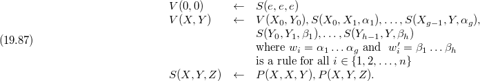
Furthermore, let  be the following conjunctive query.

Show that for the instance  of
of  that is given by
  and
and  , the tuple
  is a certain answer of query
  if and only if the Post Correspondence Problem with sets
  and
and  has no solution.
b. In contrast to the undecidability result of a., if  is a set of conjunctive views and query
  is given by datalog program
  , then it is easy to decide about an arbitrary tuple
  whether it is a certain answer of
  for a given view instance
  . Prove that the datalog program
  gives exactly the tuples of the certain answer of
  as output.
CHAPTER NOTES |
There are several dimensions along which the treatments of the problem “answering queries using views” can be classified. Figure 19.6 shows the taxonomy of the work.
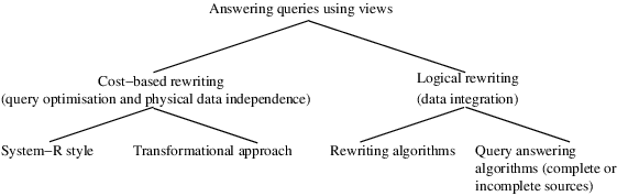
The most significant distinction between the different work s is whether their goal is data integration or whether it is query optimisation and maintenance of physical data independence. The key difference between these two classes of works is the output of the the algorithm for answering queries using views. In the former case, given a query  and a set of views
  , the goal of the algorithm is to produce an expression
  that references the views and is either equivalent to or contained in
  . In the latter case, the algorithm must go further and produce a (hopefully optimal) query execution plan for answering
  using the views (and possibly the database relations). Here the rewriting must be an equivalent to
  in order to ensure the correctness of the plan.
The similarity between these two bodies of work is that they are concerned with the core issue of whether a rewriting of a query is equivalent or contained in the query. However, while logical correctness suffices for the data integration context, it does not in the query optimisation context where we also need to find the cheapest plan using the views. The complication arises because the optimisation algorithms need to consider views that do not contribute to the logical correctness of the rewriting, but do reduce the cost of the resulting plan. Hence, while the reasoning underlying the algorithms in the data integration context is mostly logical, in the query optimisation case it is both logical and cost-based. On the other hand, an aspect stressed in data integration context is the importance of dealing with a large number of views, which correspond to data sources. In the context of query optimisation it is generally assumed (not always!) that the number of views is roughly comparable to the size of the schema.
The works on query optimisation can be classified further into System-R style optimisers and transformational optimisers. Examples of the former are works of Chaudhuri, Krishnamurty, Potomianos and Shim [61]; Tsatalos, Solomon, and Ioannidis [327]. Papers of Florescu, Raschid, and Valduriez [112]; Bello et. al. [35]; Deutsch, Popa and Tannen [89], Zaharioudakis et. al. [354], furthermore Goldstein és Larson [136] belong to the latter.
Rewriting algorithms in the data integration context are studied in works of Yang and Larson [351]; Levy, Mendelzon, Sagiv and Srivastava [155]; Qian [280]; furthermore Lambrecht, Kambhampati and Gnanaprakasam [210]. The Bucket Algorithm was introduced by Levy, Rajaraman and Ordille [156]. The Inverse-rules Algorithm is invented by Duschka and Genesereth [93], [94]. The MiniCon Algorithm was developed by Pottinger and Halevy [277], [276].
Query answering algorithms and the complexity of the problem is studied in papers of Abiteboul and Duschka [2]; Grahne and Mendelzon [140]; furthermore Calvanese, De Giacomo, Lenzerini and Vardi [54].
The STORED system was developed by Deutsch, Fernandez and Suciu [88]. Semantic caching is discussed in the paper of Yang, Karlapalem and Li [350]. Extensions of the rewriting problem are studied in [49], [110], [120], [208], [350].
Surveys of the area can be found in works of Abiteboul [1], Florescu, Levy and Mendelzon [111], Halevy [154], [153], furthermore Ullman [330].
Research of the authors was (partially) supported by Hungarian National Research Fund (OTKA) grants Nos. T034702, T037846T and T042706.
Table of Contents
The use of the internet and the development of the theory of databases mutually affect each other. The contents of web sites are usually stored by databases, while the web sites and the references between them can also be considered a database which has no fixed schema in the usual sense. The contents of the sites and the references between sites are described by the sites themselves, therefore we can only speak of semi-structured data, which can be best characterized by directed labeled graphs. In case of semi-structured data, recursive methods are used more often for giving data structures and queries than in case of classical relational databases. Different problems of databases, e.g. restrictions, dependencies, queries, distributed storage, authorities, uncertainty handling, must all be generalized according to this. Semi-structuredness also raises new questions. Since queries not always form a closed system like they do in case of classical databases, that is, the applicability of queries one after another depends on the type of the result obtained, therefore the problem of checking types becomes more emphasized.
The theoretical establishment of relational databases is closely related to finite modelling theory, while in case of semi-structured databases, automata, especially tree automata are most important.
By semi-structured data we mean a directed rooted labeled graph. The root is a special node of the graph with no entering edges. The nodes of the graph are objects distinguished from each other using labels. The objects are either atomic or complex. Complex objects are connected to one or more objects by directed edges. Values are assigned to atomic objects. Two different models are used: either the vertices or the edges are labeled. The latter one is more general, since an edge-labeled graph can be assigned to all vertex-labeled graphs in such a way that the label assigned to the edge is the label assigned to its endpoint. This way we obtain a directed labeled graph for which all inward directed edges from a vertex have the same label. Using this transformation, all concepts, definitions and statements concerning edge-labeled graphs can be rewritten for vertex-labeled graphs.
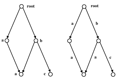
The following method is used to gain a vertex-labeled graph from an edge-labeled graph. If edge  has label
  , then remove this edge, and introduce a new vertex
  with label
  , then add edges
  and
and  . This way we can obtain a vertex-labeled graph of
  nodes and
  edges from an edge-labeled graph of
  vertices and
  edges. Therefore all algorithms and cost bounds concerning vertex-labeled graphs can be rewritten for edge-labeled graphs.
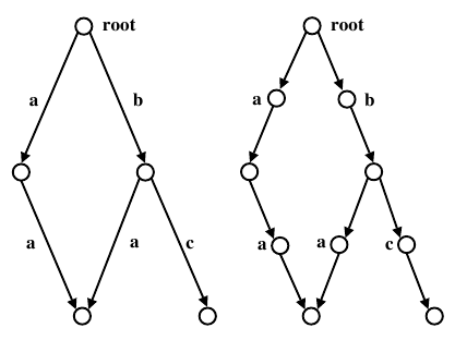
Since most books used in practice use vertex-labeled graphs, we will also use vertex-labeled graphs in this chapter.
The XML (eXtensible Markup Language) language was originally designed to describe embedded ordered labeled elements, therefore it can be used to represent trees of semi-structured data. In a wider sense of the XML language, references between the elements can also be given, thus arbitrary semi-structured data can be described using the XML language.
The medusa.inf.elte.hu/forbidden site written in XML language is as follows. We can obtain the vertex-labeled graph of Figure 20.3 naturally from the structural characteristics of the code.
       <HTML>
          <HEAD>
             <TITLE>403 Forbidden</TITLE>
          </HEAD>
          <BODY>
             <H1>Forbidden</H1>
             You don't have permission to access /forbidden.
          <ADDRESS>Apache Server at medusa.inf.elte.hu </ADDRESS>
          </BODY>
       </HTML>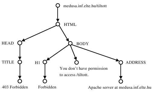
Exercises
20.1-1 Give a vertex-labeled graph that represents the structure and formatting of this chapter.
20.1-2 How many different directed vertex-labeled graphs exist with  vertices,
  edges and
  possible labels? How many of these graphs are not isomorphic? What values can be obtained for
  ,
,  and
and  ?
?
20.1-3 Consider a tree in which all children of a given node are labeled with different numbers. Prove that the nodes can be labeled with pairs  , where
  and
and  are natural numbers, in such a way that
a.  for every node
  .
.
b. If  is a descendant of
  , then
  .
.
c. If  and
and  are siblings and
  , then
  .
.
In case of relational databases, schemas play an important role in coding and querying data, query optimization and storing methods that increase efficiency. When working with semi-structured databases, the schema must be obtained from the graph. The schema restricts the possible label strings belonging to the paths of the graph.
Figure 20.4 shows the relational schemas with relations  and
and  , respectively, and the corresponding semi-structured description. The labels of the leaves of the tree are the components of the tuples. The directed paths leading from the root to the values contain the label strings database.R.tuple.A, database.R.tuple.B, database.R.tuple.C, database.Q.tuple.C, database.Q.tuple.D. This can be considered the schema of the semi-structured database. Note that the schema is also a graph, as it can be seen on Figure 20.5. The disjoint union of the two graphs is also a graph, on which a simulation mapping can be defined as follows. This way we create a connection between the original graph and the graph corresponding to the schema.
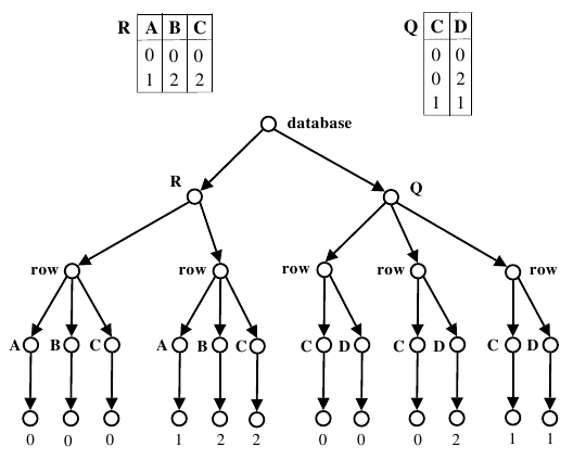
Definition 20.1 Let  be a vertex-labeled directed graph, where
  denotes the set of nodes,
  the set of edges,
  the set of labels, and
  is the label belonging to node
  . Denote by
  the set of the start nodes of the edges leading to node
  . A binary relation
  (
( ) is a simulation, if, for
  ,
,
i)  and
and
ii) for all  there exists a
  such that
Node v simulates node u, if there exists a simulation  such that
  . Node u and node v are similar,
  , if
, if  simulates
  and
and  simulates
  .
.
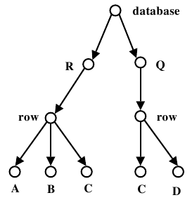
It is easy to see that the empty relation is a simulation, that the union of simulations is a simulation, that there always exists a maximal simulation and that similarity is an equivalence relation. We can write  instead of
  in the above definition, since that only means that the direction of the edges of the graph is reversed.
We say that graph  simulates graph
  if there exists a mapping
  such that the relation
  is a simulation on the set
  .
.
Two different schemas are used, a lower bound and an upper bound. If the data graph  simulates the schema graph
  , then S is a lower bound of D. Note that this means that all label strings belonging to the directed paths in
  appear in
  at some directed path. If
  simulates
  , then S is an upper bound of D. In this case, the label strings of
  also appear in
  .
.
In case of semi-structured databases, the schemas which are greatest lower bounds or lowest upper bounds play an important role.
A map between graphs  and
and  that preserves edges is called a morphism. Note that
  is a morphism if and only if
  simulates
  . To determine whether a morphism from
  to
to  exists is an NP-complete problem. We will see below, however, that the calculation of a maximal simulation is a PTIME problem.
Denote by  the nodes that simulate
  . The calculation of the maximal simulation is equivalent to the determination of all sets
  for
for  . First, our naive calculation will be based on the definition.
Naive-Maximal-Simulation(
)
1FORall2
DO3
WHILE4
DO5
RETURN
Claim 20.2 The algorithm Naive-Maximal-Simulation computes the maximal simulation in  time if
  .
.
Proof. Let us start with the elements of  . If an element
  of
of  does not simulate
  by definition according to edge
  , then we remove
  from set
  . In this case, we say that we improved set
  according to edge
  . If set
  cannot be improved according to any of the edges, then all elements of
  simulate
  . To complete the proof, notice that the
 wHILE cycle consists of at most  iterations.
The efficiency of the algorithm can be improved using special data structures. First, introduce a set  , which contains
  , and of the elements of whom we want to find out whether they simulate
  .
.
Improved-Maximal-Simulation(
)
1FORall2
DO3
IF4
THEN5
ELSE6
WHILE7
DO8
FORall9
DO10
11
RETURN
The wHILE cycle of the improved algorithm possesses the following invariant characteristics.
 :
:  .
.
 :
: 
 .
.
When improving the set  according to edge
  , we check whether an element
  has parents in
  . It is sufficient to check that for the elements of
  instead of
  because of
  . Once an element
  was chosen, it is removed from set
  .
.
We can further improve the algorithm if we do not compute the set  in the iterations of the
 wHILE cycle but refresh the set dynamically.
Efficient-Maximal-Simulation(
)
1FORall2
DO3
IF4
THEN5
ELSE6
7
WHILE8
DOFORall9
DOFORall10
DOIF11
THEN12
FORall13
DOIF14
THEN
15
16
17
RETURN
The above algorithm possesses the following invariant characteristic with respect to the wHILE cycle.
 :
:  :
:  .
.
Use an  array as a counter for the realization of the algorithm. Let the value
  be the nonnegative integer
  . The initial values of the counter are set in
  time. When element
  is removed from set
  , the values
  must be decreased for all children
  of
of  . By this we ensure that the innermost
 iF condition can be checked in constant time. At the beginning of the algorithm, the initial values of the sets  are set in
  time if
  . The setting of sets
  takes altogether
  time. For arbitrary nodes
  and
and  , if
, if  is true in the
  -th iteration of the
 wHILE cycle, then it will be false in the  -th iteration for
  . Since
  implies
  , the value of
  in the
  -th iteration is a subset of the value of
  in the
  -th iteration, and we know that invariant
  holds. Therefore
  can be checked in
  time.
time.  is true at most once for all nodes
  and
and  , since once the condition holds, we remove
  from set
  . This implies that the computation of the outer
 iF condition of the wHILE cycle takes  time.
time.
Thus we have proved the following proposition.
Claim 20.3 The algorithm Effective-Maximal-Simulation computes the maximal simulation in  time if
  .
.
If the inverse of a simulation is also a simulation, then it is called a bisimulation. The empty relation is a bisimulation, and there always exist a maximal bisimulation. The maximal bisimulation can be computed more efficiently than the simulation. The maximal bisimulation can be computed in  time using the
 PT algorithm. In case of edge-labeled graphs, the cost is  .
.
We will see that bisimulations play an important role in indexing semi-structured databases, since the quotient graph of a graph with respect to a bisimulation contains the same label strings as the original graph. Note that in practice, instead of simulations, the so-called DTD descriptions are also used as schemas. DTD consists of data type definitions formulated in regular language.
Exercises
20.2-1 Show that simulation does not imply bisimulation.
20.2-2 Define the operation turn-tree for a directed, not necessarily acyclic, vertex-labeled graph  the following way. The result of the operation is a not necessarily finite graph
  , the vertices of which are the directed paths of
  starting from the root, and the labels of the paths are the corresponding label strings. Connect node
  with node
  by an edge if
  can be obtained from
  by deletion of its endpoint. Prove that
  and
and  are similar with respect to the bisimulation.
The information stored in semi-structured databases can be retrieved using queries. For this, we have to fix the form of the questions, so we give a query language, and then define the meaning of questions, that is, the query evaluation with respect to a semi-structured database. For efficient evaluation we usually use indexes. The main idea of indexing is that we reduce the data stored in the database according to some similarity principle, that is, we create an index that reflects the structure of the original data. The original query is executed in the index, then using the result we find the data corresponding to the index values in the original database. The size of the index is usually much smaller than that of the original database, therefore queries can be executed faster. Note that the inverted list type index used in case of classical databases can be integrated with the schema type indexes introduced below. This is especially advantageous when searching XML documents using keywords.
First we will get acquainted with the query language consisting of regular expressions and the index types used with it.
Definition 20.4 Given a directed vertex-labeled graph  , where
  denotes the set of vertices,
  the set of edges and
  the set of labels.
  contains two special labels, ROOT and VALUE. The label of vertex
  is
is  , and the identifier of vertex
  is
is  . The root is a node with label ROOT, and from which all nodes can be reached via directed paths. If
  is a leaf, that is, if it has no outgoing edges, then its label is VALUE, and
  is the value corresponding to leaf
  . Under the term path we always mean a directed path, that is, a sequence of nodes
  such that there is an edge from
  to
to  if
if  . A sequence of labels
  is called a label sequence or simple expression. Path
  fits to the label sequence
  if
if  for all
  .
.
We define regular expressions recursively.
Definition 20.5 Let  , where R is a regular expression, and
  is the empty expression, _ denotes an arbitrary label, . denotes succession, | is the logical OR operation, ? is the optional choice, and * means finite repetition. Denote by L(R) the regular language consisting of the label sequences determined by
  . Node n fits to a label sequence if there exists a path from the root to node
  such that fits to the label sequence. Node
  fits to the regular expression
  if there exists a label sequence in the language
  , to which node
  fits. The result of the query on graph G determined by the regular expression
  is the set
  of nodes that fit to expression
  .
.
Since we are always looking for paths starting from the root when evaluating regular expressions, the first element of the label sequence is always ROOT, which can therefore be omitted.
Note that the set of languages  corresponding to regular expressions is closed under intersection, and the problem whether
  is decidable.
The result of the queries can be computed using the nondeterministic automaton  corresponding to the regular expression
  . The algorithm given recursively is as follows.
Naive-Evaluation(
)
  1         If we were in node  in state , then  was put in set Visited.
  2  Traverse()

Traverse(
)
1IFVisited 2
THENRETURN3
4
5
FORall
If we get to state
from state
by reading sign
. 6
DOIF7
THEN8
Traverse()9FORall
If we get to state
from state
by reading sign
. 10
DOIF11
THEN12
FORall, where

Continue the traversal for the children of node
recursively. 13
DOTraverse()14RETURN


Claim 20.6 Given a regular query  and a graph
  , the calculation cost of
  is a polynomial of the number of edges of
  and the number of different states of the finite nondeterministic automaton corresponding to
  .
.
Proof. The sketch of the proof is the following. Let  be the finite nondeterministic automaton corresponding to
  . Denote by
  the number of states of
  . Consider the breadth-first traversal corresponding to the algorithm
 Traverse of graph  with
with  edges, starting from the root. During the traversal we get to a new state of the automaton according to the label of the node, and we store the state reached at the node for each node. If the final state of the automaton is acceptance, then the node is a result. During the traversal, we sometimes have to step back on an edge to ensure we continue to places we have not seen yet. It can be proved that during a traversal every edge is used at most once in every state, so this is the number of steps performed by that automaton. This means
  steps altogether, which completes the proof.
Two nodes of graph  are indistinguishable with regular expressions if there is no regular
  for which one of the nodes is among the results and the other node is not. Of course, if two nodes cannot be distinguished, then their labels are the same. Let us categorize the nodes in such a way that nodes with the same label are in the same class. This way we produce a partition
  of the set of nodes, which is called the basic partition. It can also be seen easily that if two nodes are indistinguishable, then it is also true for the parents. This implies that the set of label sequences corresponding to paths from the root to the indistinguishable nodes is the same. Let
  for all nodes
  . Nodes
  and
and  are indistinguishable if and only if
  . If the nodes are assigned to classes in such a way that the nodes having the same value
  are arranged to the same class, then we get a refinement
  of partition
  . For this new partition, if a node
  is among the results of a regular query
  , then all nodes from the equivalence class of
  are also among the results of the query.
Definition 20.7 Given a graph  and a partition
  of
of  that is a refinement of the basic partition, that is, for which the nodes belonging to the same equivalence class have the same label. Then the graph
  is called an index. The nodes of the index graph are the equivalence classes of partition
  , and
, and  if and only if there exist
  and
and  such that
  . If
. If  , then
  is the identifier of index node
  ,
,  , where
  , and root' is the equivalence class of partition
  that contains the root of
  . If
. If  , then
  .
.
Given a partition  of set
  , denote by class(n) the equivalence class of
  that contains
  for
for  . In case of indexes, the notation
  can also be used instead of
  .
.
Note that basically the indexes can be identified with the different partitions of the nodes, so partitions can also be called indexes without causing confusion. Those indexes will be good that are of small size and for which the result of queries is the same on the graph and on the index. Indexes are usually given by an equivalence relation on the nodes, and the partition corresponding to the index consists of the equivalence classes.
Definition 20.8 Let  be the partition for which
  for a class
  if and only if
  . Then the index
  corresponding to
  is called a naive index.
In case of naive indexes, the same language  is assigned to all elements
  of class
  in partition
  , which will be denoted by
  .
.
Claim 20.9 Let  be a node of the naive index and
  a regular expression. Then
  or
or  .
.
Proof. Let  and
and  . Then there exists a label sequence
  in
in  to which
  fits, that is,
  . Since
  ,
,  also fits to this label sequence, so
  .
.
Naive-Index-Evaluation(
)
1 letbe the naive index of
2
3
FORall4
DO5
RETURN
Claim 20.10 Set  produced by the algorithm
 Naive-Index-Evaluation is equal to  .
.
Proof. Because of the previous proposition either all elements of a class  are among the results of a query or none of them.
Using naive indexes we can evaluate queries, but, according to the following proposition, not efficiently enough. The proposition was proved by Stockmeyer and Meyer in 1973.
Claim 20.11 The creation of the naive index  needed in the algorithm
 Naive-Index-Evaluation is PSPACE-complete.
The other problem with using naive indexes is that the sets  are not necessary disjoint for different
  , which might cause redundancy in storing.
Because of the above we will try to find a refinement of the partition corresponding to the naive index, which can be created efficiently and can still be used to produce  .
.
Definition 20.12 Index  is safe if for any
  and label sequence
  such that
  fits to the label sequence
  in graph
  , class(
 ) fits to the label sequence
  in graph
  . Index
  is exact if for any class
  of the index and label sequence
  such that
  fits to the label sequence
  in graph
  , arbitrary node
  fits to the label sequence
  in graph
  .
.
Safety means that the nodes belonging to the result we obtain by evaluation using the index contain the result of the regular query, that is,  , while exactness means that the evaluation using the index does not provide false results, that is,
  . Using the definitions of exactness and of the edges of the index the following proposition follows.
Claim 20.13 1. Every index is safe.
2. The naive index is safe and exact.
If  is a set of nodes of
  , then the language
  , to the label strings of which the elements of
  fit, was defined using graph
  . If we wish to indicate this, we use the notation
  . However,
  can also be defined using graph
  , in which
  is a node. In this case, we can use the notation
  instead of
  , which denotes all label sequences to which node
  fits in graph
  .
.  for safe and exact indexes, so in this case we can write
  for simplicity. Then
  can be computed using
  , since the size of
  is usually smaller than that of
  .
.
Arbitrary index graph can be queried using the algorithm Naive-Evaluation. After that join the index nodes obtained. If we use an exact index, then the result will be the same as the result we would have obtained by querying the original graph.
Index-Evaluation(
)
1 letbe the index of
2
3
FORall4
DO5
RETURN
First, we will define a safe and exact index that can be created efficiently, and is based on the similarity of nodes. We obtain the 1-index this way. Its size can be decreased if we only require similarity locally. The A( )-index obtained this way lacks exactness, therefore using the algorithm
 Index-Evaluation we can get results that do not belong to the result of the regular query  , so we have to test our results to ensure exactness.
Definition 20.14 Let  be an equivalence relation on set
  such that, for
  ,
,
i)  ,
,
ii) if there is an edge from node  to node
  , then there exists a node
  for which there is an edge from node
  to node
  and
and  .
.
iii) if there is an edge from node  to node
  , then there exists a node
  for which there is an edge from node
  to node
  and
and  .
.
The above equivalence relation is called a bisimulation. Nodes  and
and  of a graph are bisimilar if and only if there exists a bisimulation
  such that
  .
.
Definition 20.15 Let  be the partition consisting of the equivalence classes of a bisimulation. The index defined using partition
  is called 1-index.
Claim 20.16 The 1-index is a refinement of the naive index. If the labels of the ingoing edges of the nodes in graph  are different, that is,
  for
for  and
and  , then
  if and only if
  and
and  are bisimilar.
Proof.  if
if  . Let node
  fit to the label sequence
  , and let
  be the node corresponding to label
  . Then there exists a
  such that
  and
and  .
.  fits to the label sequence
  , so, by induction,
  also fits to the label sequence
  , therefore
  fits to the label sequence
  . So, if two nodes are in the same class according to the 1-index, then they are in the same class according to the naive index as well.
To prove the second statement of the proposition, it is enough to show that the naive index corresponds to a bisimulation. Let  and
and  be in the same class according to the naive index. Then
  . If
. If  , then there exists a label sequence
  such that the last two nodes corresponding to the labels are
  and
and  . Since we assumed that the labels of the parents are different,
  , where
  and
and  are disjoint, and
  fits to the sequence
  , and
, and  , while
  . Since
  , there exists a
  such that
  and
and  .
.  fits to the sequence
  , and
, and  because of the different labels of the parents, so
  , and
, and  by induction, therefore
  .
.
Claim 20.17 The 1-index is safe and exact.
Proof. If  fits to the label sequence
  in graph
  because of nodes
  , then, by the definition of the index graph, there exists an edge from
  to
to  ,
,  , that is,
  fits to the label sequence
  in graph
  . To prove exactness, assume that
  fits to the label sequence
  in graph
  because of
  . Then there are
  ,
,  such that
  and
and  , that is,
  . We can see by induction that
  fits to the label sequence
  because of nodes
  , but then
  fits to the label sequence
  because of nodes
  in graph
  .
.
If we consider the bisimulation in case of which all nodes are assigned to different partitions, then the graph  corresponding to this 1-index is the same as graph
  . Therefore the size of
  is at most the size of
  , and we also have to store the elements of
  for the nodes
  of
of  , which means we have to store all nodes of
  . For faster evaluation of queries we need to find the smallest 1-index, that is, the coarsest 1-index. It can be checked that
  and
and  are in the same class according to the coarsest 1-index if and only if
  and
and  are bisimilar.
1-Index-Evaluation(
)
1 letbe the coarsest 1-index of
2
RETURNIndex-Evaluation()

In the first step of the algorithm, the coarsest 1-index has to be given. This can be reduced to finding the coarsest stable partition, what we will discuss in the next section of this chapter. Thus using the efficient version of the PT-algorithm, the coarsest 1-index can be found with computation cost  and space requirement
  , where
  and
and  denote the number of nodes and edges of graph
  , respectively.
Since graph  is safe and exact, it is sufficient to evaluate the query in graph
  , that is, to find the index nodes that fit to the regular expression
  . Using Proposition 20.6, the cost of this is a polynomial of the size of graph
  .
.
The size of  can be estimated using the following parameters. Let
  be the number of different labels in graph
  , and
, and  the diameter of graph
  , that is, the length of the longest directed path. (No node can appear twice in the directed path.) If the graph is a tree, then the diameter is the depth of the tree. We often create websites that form a tree of depth
  , then we add a navigation bar consisting of
  elements to each page, that is, we connect each node of the graph to
  chosen pages. It can be proved that in this case the diameter of the graph is at most
  . In practice,
  and
and  are usually very small compared to the size of the graph. The proof of the following proposition can be found in the paper of Milo and Suciu.
Claim 20.18 Let the number of different labels in graph  be at most
  , and let the diameter of
  be less than
  . Then the size of the 1-index
  defined by an arbitrary bisimulation can be bounded from above with a bound that only depends on
  and
and  but does not depend on the size of
  .
.
Exercises
20.3-1 Show that the index corresponding to the maximal simulation is between the 1-index and the naive index with respect to refinement. Give an example that shows that both inclusions are proper.
20.3-2 Denote by  the index corresponding to the maximal simulation. Does
  hold?
hold?
20.3-3 Represent graph  and the state transition graph of the automaton corresponding to the regular expression
  with relational databases. Give an algorithm in a relational query language, for example in PL/SQL, that computes
  .
.
Most index structures used for efficient evaluation of queries of semi-structured databases are based on a partition of the nodes of a graph. The problem of creating indexes can often be reduced to finding the coarsest stable partition.
Definition 20.19 Let  be a binary relation on the finite set
  , that is,
  . Then
  is the set of nodes, and
  is the set of edges. For arbitrary
  , let
, let  and
and  . We say that
  is stable with respect to
  for arbitrary
  and
and  , if
, if  or
or  . Let
. Let  be a partition of
  , that is, a decomposition of
  into disjoint sets, or in other words, blocks. Then
  is stable with respect to
  , if all blocks of
  are stable with respect to
  .
.  is stable with respect to partition
  , if all blocks of
  are stable with respect to all blocks of
  . If
. If  is stable with respect to all of its blocks, then partition
  is stable. Let
  and
and  be two partitions of
  .
.  is a refinement of
  , or
, or  is coarser than
  , if every block of
  is the union of some blocks of
  . Given
  ,
,  and
and  , the coarsest stable partition is the coarsest stable refinement of
  , that is, the stable refinement of
  that is coarser than any other stable refinement of
  .
.
Note that stability is sometimes defined the following way.  is stable with respect to
  if
if  or
or  . This is not a major difference, only the direction of the edges is reversed. So in this case stability is defined with respect to the binary relation
  instead of
  , where
  if and only if
  , since
  .
.
Let  and
and  . We will prove that there always exists a unique solution of the problem of finding the coarsest stable partition, and there is an algorithm that finds the solution in
  time with space requirement
  . This algorithm was published by R. Paige and R. E. Tarjan in 1987, therefore it will be called the PT-algorithm.
The main idea of the algorithm is that if a block is not stable, then it can be split into two in such a way that the two parts obtained are stable. First we will show a naive method. Then, using the properties of the split operation, we will increase its efficiency by continuing the procedure with the smallest part.
Definition 20.20 Let  be a binary relation on
  ,
,  and
and  a partition of
  . Furthermore, let split(
 ) be the refinement of
  which is obtained by splitting all blocks
  of
of  that are not disjoint from
  , that is,
  and
and  . In this case, add blocks
  and
and  to the partition instead of
  .
.  is a splitter of
  if
if  .
.
Note that  is not stable with respect to
  if and only if
  is a splitter of
  .
.
Stability and splitting have the following properties, the proofs are left to the Reader.
Claim 20.21 Let  and
and  be two subsets of
  , while
  and
and  two partitions of
  . Then
1. Stability is preserved under refinement, that is, if  is a refinement of
  , and
, and  is stable with respect to
  , then
  is also stable with respect to
  .
.
2. Stability is preserved under unification, that is, if  is stable with respect to both
  and
and  , then
  is stable with respect to
  .
.
3. The split operation is monotonic in its second argument, that is, if  is a refinement of
  , then split(
 ) is a refinement of split(
 ).
).
4. The split operation is commutative in the following sense. For arbitrary  ,
,  and
and  , split(
 , split(
 )) = split(
 , split(
 )), and the coarsest partition of
  that is stable with respect to both
  and
and  is split(
 , split(
 )).
)).
In the naive algorithm, we refine partition  starting from partition
  , until
  is stable with respect to all of its blocks. In the refining step, we seek a splitter
  of
of  that is a union of some blocks of
  . Note that finding a splitter among the blocks of
  would be sufficient, but this more general way will help us in improving the algorithm.
Naive-PT(
)
12
WHILEis not stable 3
DOletbe a splitter of
that is the union of some blocks of
4
5
RETURN
Note that the same set  cannot be used twice during the execution of the algorithm, since stability is preserved under refinement, and the refined partition obtained in step 4 is stable with respect to
  . The union of the sets
  used can neither be used later, since stability is also preserved under unification. It is also obvious that a stable partition is stable with respect to any
  that is a union of some blocks of the partition. The following propositions can be proved easily using these properties.
Claim 20.22 In any step of the algorithm Naive-PT, the coarsest stable refinement of  is a refinement of the actual partition stored in
  .
.
Proof. The proof is by induction on the number of times the cycle is executed. The case  is trivial. Suppose that the statement holds for
  before using the splitter
  . Let
. Let  be the coarsest stable refinement of
  . Since
  consists of blocks of
  , and, by induction,
  is a refinement of
  , therefore
  is the union of some blocks of
  .
.  is stable with respect to all of its blocks and the union of any of its blocks, thus
  is stable with respect to
  , that is,
  . On the other hand, using that the split operation is monotonic,
  is a refinement of
  , which is the actual value of
  .
.
Claim 20.23 The algorithm Naive-PT determines the unique coarsest stable refinement of  , while executing the cycle at most
  times.
Proof. The number of blocks of  is obviously at least
  and at most
  . Using the split operation, at least one block of
  is divided into two, so the number of blocks increases. This implies that the cycle is executed at most
  times.
  is a stable refinement of
  when the algorithm terminates, and, using the previous proposition, the coarsest stable refinement of
  is a refinement of
  . This can only happen if
  is the coarsest stable refinement of
  .
.
Claim 20.24 If we store the set  for all elements
  of
of  , then the cost of the algorithm
 Naive-PT is at most  .
.
Proof. We can assume, without restricting the validity of the proof, that there are no sinks in the graph, that is, every node has outgoing edges. Then  for arbitrary
  in
in  . Consider a partition
  , and split all blocks
  of
of  . Let
. Let  be the set of the nodes of
  that have at least one outgoing edge. Then
  . Now let
  , that is, the set of sinks of
  . Set
. Set  is stable with respect to arbitrary
  , since
  , so
, so  does not have to be split during the algorithm. Therefore, it is enough to examine partition
  consisting of blocks
  instead of
  , that is, a partition of set
  . By adding blocks
  to the coarsest stable refinement of
  we obviously get the coarsest stable refinement of
  . This means that there is a preparation phase before the algorithm in which
  is obtained, and a processing phase after the algorithm in which blocks
  are added to the coarsest stable refinement obtained by the algorithm. The cost of preparation and processing can be estimated the following way.
  has at most
  elements. If, for all
  in
in  we have
  , then the preparation and processing requires
  time.
time.
From now on we will assume that  holds for arbitrary
  in
in  , which implies that
  . Since we store sets
  , we can find a splitter among the blocks of partition
  in
in  time. This, combined with the previous proposition, means that the algorithm can be performed in
  time.
time.
The algorithm can be executed more efficiently using a better way of finding splitter sets. The main idea of the improved algorithm is that we work with two partitions besides  ,
,  and a partition
  that is a refinement of
  in every step such that
  is stable with respect to all blocks of
  . At the start, let
  and let
  be the partition consisting only one block, set
  . The refining step of the algorithm is repeated until
  .
.
PT(
)
12
3
WHILE4
DOletbe a block of
that is not a block of
, and
a block of
in
for which
5
6
7
RETURN
Claim 20.25 The result of the PT-algorithm is the same as that of algorithm Naive-PT.
Proof. At the start,  is a stable refinement of
  with respect to the blocks of
  . In step 5, a block of
  is split, thus we obtain a refinement of
  . In step 6, by refining
  using splits we ensure that
  is stable with respect to two new blocks of
  . The properties of stability mentioned in Proposition 20.21 and the correctness of algorithm
 Naive-PT imply that the PT-algorithm also determines the unique coarsest stable refinement of  .
.
In some cases one of the two splits of step 6 can be omitted. A sufficient condition is that  is a function of
  .
.
Claim 20.26 If  for all
  in
in  , then step 6 of the
 PT-algorithm can be exchanged with  .
.
Proof. Suppose that  is stable with respect to a set
  which is the union of some blocks of
  . Let
. Let  be a block of
  that is a subset of
  . It is enough to prove that
  is stable with respect to
  . Let
. Let  be a block of
  . Since the result of a split according to
  is a stable partition with respect to
  , either
  or
or  . Using
  , we get
  in the first case, and
  in the second case, which means that we obtained a stable partition with respect to
  .
.
Note that the stability of a partition with respect to  and
and  generally does not imply that it is also stable with respect to
  . If this is true, then the execution cost of the algorithm can be reduced, since the only splits needed are the ones according to
  because of the reduced sizes.
The two splits of step 6 can cut a block into four parts in the general case. According to the following proposition, one of the two parts gained by the first split of a block remains unchanged at the second split, so the two splits can result in at most three parts. Using this, the efficiency of the algorithm can be improved even in the general case.
Claim 20.27 Let  be a stable partition with respect to
  , where
  is the union of some blocks of
  , and let
  be a block of
  that is a subset of
  . Furthermore, let
  be a block of
  that is cut into two (proper) parts
  and
and  by the operation
  in such a way that none of these is the empty set. Suppose that block
  is further divided into the nonempty sets
  and
and  by
by  . Then
1.  and
and  if and only if
  and
and  .
.
2.  and
and  if and only if
  and
and  .
.
3. The operation  leaves block
  unchanged.
4.  .
.
Proof. The first two statements follow using the definition of the split operation. To prove the third statement, suppose that  was obtained from
  by a proper decomposition. Then
  , and since
  ,
,  . All blocks of partition
  , including
  , are stable with respect to
  , which implies
  . Since
  ,
,  using the first statement, so
  is stable with respect to the set
  , therefore a split according to
  does not divide block
  . Finally, the fourth statement follows from
  and
and  .
.
Denote by  the number of nodes in
  that can be reached from
  , that is,
  . Note that if
  , then
  .
.
Since sizes are always halved, an arbitrary  in
in  can appear in at most
  different sets
  that were used for refinement in the
 PT-algorithm. In the following, we will give an execution of the PT algorithm in which the determination of the refinement according to block  in steps 5 and 6 of the algorithm costs
  . Summing this for all blocks
  used in the algorithm and for all elements of these blocks, we get that the complexity of the algorithm
 Efficient-PT is at most  . To give such a realization of the algorithm, we have to choose good data structures for the representation of our data.
-
Attach node
 to all edges
  of set
  , and attach the list
  to all nodes
  . Then the cost of reading set
  is proportional to the size of
  .
. -
Let partition
 be a refinement of partition
  . Represent the blocks of the two partitions by records. A block
  of partition
  is simple if it consists of one block of
  , otherwise it is compound.
 -
Let
 be the list of all compound blocks in partition
  . At start, let
  , since
  is the union of the blocks of
  . If
. If  consists of only one block, then
  is its own coarsest stable refinement, so no further computation is needed.
 -
For any block
 of partition
  , let Q-blocks(
 ) be the double-chained list of the blocks of partition
  the union of which is set
  . Furthermore, store the values
  for all
  in set
  to which one pointer points from all edges
  such that
  is an element of
  . At start, the value assigned to all nodes
  is
is  , and make a pointer to all nodes
  that points to the value
  .
. -
For any block
 of partition
  , let X-block(
 ) be the block of partition
  in which
  appears. Furthermore, let
  be the cardinality of
  , and
, and  the double-chained list of the elements of
  . Attach a pointer to all elements that points to the block of
  in which this element appears. Using double chaining any element can be deleted in
  time.
time.
Using the proof of Proposition 20.24, we can suppose that  without restricting the validity. It can be proved that in this case the space requirement for the construction of such data structures is
  .
.
Efficient-PT(
)
1IF2
THENRETURN3
4
5


is the list of the compound blocks of
. 6
WHILE7
DOletbe an element of
8 let
be the smaller of the first two elements of
9
10
11
12
IF13
THEN14 Generate set
by reading the edges
of set
for which
is an element of
, and for all elements
of this set, compute the value
. 15 Find blocks
and
for all blocks
of
by reading set
16 By reading all edges
of set
for which
is an element of
, create set
checking the condition
17 Reading set
, for all blocks
of
, determine the sets
and
18
FORall blocksof
for which
,
and
19
DOIFis a simple block of
20
THEN21
22 Compute the value
by reading the edges
of
for which
is an element of
. 23
RETURN
Claim 20.28 The algorithm Efficient-PT determines the coarsest stable refinement of  . The computation cost of the algorithm is
  , and its space requirement is
  .
.
Proof. The correctness of algorithm follows from the correctness of the PT-algorithm and Proposition 20.27. Because of the data structures used, the computation cost of the steps of the cycle is proportional to the number of edges examined and the number of elements of block  , which is
  altogether. Sum this for all blocks
  used during the refinement and all elements of these blocks. Since the size of
  is at most half the size of
  , arbitrary
  in set
  can be in at most
  different sets
  . Therefore, the total computation cost of the algorithm is
  . It can be proved easily that a space of
  size is enough for the storage of the data structures used in the algorithm and their maintenance.
Note that the algorithm could be further improved by contracting some of its steps but that would only decrease computation cost by a constant factor.
Let  be the graph that can be obtained from
  by changing the direction of all edges of
  . Consider a 1-index in graph
  determined by the bisimulation
  . Let
. Let  and
and  be two classes of the bisimulation, that is, two nodes of
  . Using the definition of bisimulation,
  or
or  . Since
  , this means that
  is stable with respect to
  in graph
  . So the coarsest 1-index of
  is the coarsest stable refinement of the basic partition of graph
  .
.
Corollary 20.29 The coarsest 1-index can be determined using the algorithm Efficient-PT. The computation cost of the algorithm is at most  , and its space requirement is at most
  .
.
Exercises
20.4-1 Prove Proposition 29.21.
20.4-2 Partition  is size-stable with respect to set
  if
if  for arbitrary elements
  ,
,  of a block
  of
of  . A partition is size-stable if it is size-stable with respect to all its blocks. Prove that the coarsest size-stable refinement of an arbitrary partition can be computed in
  time.
time.
20.4-3 The 1-index is minimal if no two nodes  and
and  with the same label can be contracted, since there exists a node
  for which
  is not stable with respect to
  . Give an example that shows that the minimal 1-index is not unique, therefore it is not the same as the coarsest 1-index.
20.4-4 Prove that in case of an acyclic graph, the minimal 1-index is unique and it is the same as the coarsest 1-index.
In case of 1-indexes, nodes of the same class fit to the same label sequences starting from the root. This means that the nodes of a class cannot be distinguished by their ancestors. Modifying this condition in such a way that indistinguishability is required only locally, that is, nodes of the same class cannot be distinguished by at most  generations of ancestors, we obtain an index that is coarser and consists of less classes than the 1-index. So the size of the index decreases, which also decreases the cost of the evaluation of queries. The 1-index was safe and exact, which we would like to preserve, since these guarantee that the result we get when evaluating the queries according to the index is the result we would have obtained by evaluating the query according to the original graph. The A(
 )-index is also safe, but it is not exact, so this has to be ensured by modification of the evaluation algorithm.
Definition 20.30 The k-bisimulation  is anequivalence relation on the nodes
  of a graph defined recursively as
i)  if and only if
  ,
,
ii)  if and only if
  and if there is an edge from node
  to node
  , then there is a node
  from which there is an edge to node
  and
and  , also, if there is an edge from node
  to node
  , then there is a node
  from which there is an edge to node
  and
and  .
.
In case 
 and
and  are k-bisimilar. The classes of the partition according to the A(
 )-index are the equivalence classes of the
  -bisimulation.
The “A” in the notation refers to the word “approximative”.
Note that the partition belonging to  is the basic partition, and by increasing
  we refine this, until the coarsest 1-index is reached.
Denote by  the label sequences of length at most
  to which
  fits in graph
  . The following properties of the A(
 )-index can be easily checked.
1. If  and
and  are
are  -bisimilar, then
  .
.
2. If  is a node of the A(
 )-index and
  , then
  .
.
3. The A( )-index is exact in case of simple expressions of length at most
  .
.
4. The A( )-index is safe.
5. The  -bisimulation is a (not necessarily proper) refinement of the
  -bisimulation.
The A( )-index compares the
  -distance half-neighbourhoods of the nodes which contain the root, so the equivalence of the nodes is not affected by modifications outside this neighbourhood, as the following proposition shows.
Claim 20.32 Suppose that the shortest paths from node  to nodes
  and
and  contain more than
  edges. Then adding or deleting an edge from
  to
to  does not change the
  -bisimilarity of
  and
and  .
.
We use a modified version of the PT-algorithm for creating the A( )-index. Generally, we can examine the problem of approximation of the coarsest stable refinement.
Definition 20.33 Let  be a partition of
  in the directed graph
  , and let
  be a sequence of partitions such that
  and
and  is the coarsest refinement of
  that is stable with respect to
  . In this case, partition
  is the
  -step approximation of the coarsest stable refinement of
  .
.
Note that every term of sequence  is a refinement of
  , and if
  , then
  is the coarsest stable refinement of
  . It can be checked easily that an arbitrary approximation of the coarsest stable refinement of
  can be computed greedily, similarly to the
 PT-algorithm. That is, if a block  of
of  is not stable with respect to a block
  of
of  , then split
  according to
  , and consider the partition
  instead of
  .
.
Naive-Approximation(
)
12
FOR
TO3
DO4
FORallsuch that
5
DO6
RETURN
Note that the algorithm Naive-Approximation could also be improved similarly to the PT-algorithm.
Algorithm Naive-Approximation can be used to compute the A( )-index, all we have to notice is that the partition belonging to the A(
 )-index is stable with respect to the partition belonging to the A(
 )-index in graph
  . It can be shown that the computation cost of the A(
 )-index obtained this way is
  , where
  is the number of edges in graph
  .
.
A(
)-Index-Evaluation(
)
1 letbe the A(
)-index of
2
Index-Evaluation()3FORall4
DOIF5
THEN6
RETURN


The A( )-index is safe, but it is only exact for simple expressions of length at most
  , so in step 4, we have to check for all elements
  of set
  whether it satisfies query
  , and we have to delete those from the result that do not fit to query
  . We can determine using a finite nondeterministic automaton whether a given node satisfies expression
  as in Proposition 20.6, but the automaton has to run in the other way. The number of these checks can be reduced according to the following proposition, the proof of which is left to the Reader.
Claim 20.34 Suppose that in the graph  belonging to the A(
 )-index, index node
  fits to a label sequence that ends with
  ,
,  . If all label sequences of the form s'.s that start from the root satisfy expression
  in graph
  , then all elements of
  satisfy expression
  .
.
Exercises
20.5-1 Denote by  the A(
 )-index of
  . Determine whether
  .
.
20.5-2 Prove Proposition 20.31.
20.5-3 Prove Proposition 20.32.
20.5-4 Prove Proposition 20.34.
20.5-5 Prove that the algorithm Naive-approximation generates the coarsest k-step stable approximation.
20.5-6 Let  be a set of indexes, the elements of which are A(
 )-, A(
 )-,
)-,  , A(
, A( )-indexes, respectively.
  is minimal, if by uniting any two elements of
  ,
,  is not stable with respect to
  ,
,  . Prove that for arbitrary graph, there exists a unique minimal
  the elements of which are coarsest A(
 )-indexes,
  .
.
When using A( )-indexes, the value of
  must be chosen appropriately. If
  is too large, the size of the index will be too big, and if
  is too small, the result obtained has to be checked too many times in order to preserve exactness. Nodes of the same class are similar locally, that is, they cannot be distinguished by their
  distance neighbourhoods, or, more precisely, by the paths of length at most
  leading to them. The same
  is used for all nodes, even though there are less important nodes. For instance, some nodes appear very rarely in results of queries in practice, and only the label sequences of the paths passing through them are examined. There is no reason for using a better refinement on the less important nodes. This suggests the idea of using the dynamic D(
 )-index, which assigns different values
  to the nodes according to queries. Suppose that a set of queries is given. If there is an
  and an
  query among them, where
  and
and  are regular queries, then a partition according to at least 1-bisimulation in case of nodes with label
  , and according to at least 2-bisimulation in case of nodes with label
  is needed.
Definition 20.35 Let  be the index graph belonging to graph
  , and to all index node
  assign a nonnegative integer
  . Suppose that the nodes of block
  are
are  -bisimilar. Let the values
  satisfy the following condition: if there is an edge from
  to
to  in graph
  , then
  . The index
  having this property is called a D(
 )-index.
The “D” in the notation refers to the word “dynamic”. Note that the A( )-index is a special case of the D(
 )-index, since in case of A(
 )-indexes, the elements belonging to any index node are exactly
  -bisimilar.
Since classification according to labels, that is, the basic partition is an A( )-index, and in case of finite graphs, the 1-index is the same as an A(
 )-index for some
  , these are also special cases of the D(
 )-index. The D(
 )-index, just like any other index, is safe, so it is sufficient to evaluate the queries on them. Results must be checked to ensure exactness. The following proposition states that exactness is guaranteed for some queries, therefore checking can be omitted in case of such queries.
Claim 20.36 Let  be a directed path in the D(
 )-index, and suppose that
  if
if  . Then all elements of
  fit to the label sequence
  .
.
Proof. The proof is by induction on  . The case
  is trivial. By the inductive assumption, all elements of
  fit to the label sequence
  . Since there is an edge from node
  to node
  in graph
  , there exist
  and
and  such that there is an edge from
  to
to  in graph
  . This means that
  fits to the label sequence
  of length
  . The elements of
  are at least
  -bisimilar, therefore all elements of
  fit to this label sequence.
Corollary 20.37 The D( )-index is exact with respect to label sequence
  if
if  for all nodes
  of the index graph that fit to this label sequence.
When creating the D( )-index, we will refine the basic partition, that is, the A(
 )-index. We will assign initial values to the classes consisting of nodes with the same label. Suppose we use
  different values. Let
  be the set of these values, and denote the elements of
  by
by  . If the elements of
  do not satisfy the condition given in the D(
 )-index, then we increase them using the algorithm
 Weight-Changer, starting with the greatest value, in such a way that they satisfy the condition. Thus, the classes consisting of nodes with the same label will have good  values. After this, we refine the classes by splitting them, until all elements of a class are
  -bisimilar, and assign this
  to all terms of the split. During this process the edges of the index graph must be refreshed according to the partition obtained by refinement.
Weight-Changer(
)
12
3
WHILE4
DOFORall, where
is a node of the A(
)-index and
5
DOFORall, where
is a node of the A(
)-index and there is an edge from
to
6
7
8
9
RETURN
It can be checked easily that the computation cost of the algorithm Weight-Changer is  , where
  is the number of edges of the A(
 )-index.
D(
)-Index-Creator(
)
1 letbe the A(
)-index belonging to graph
, let
be the set of nodes of
, let
be the set of edges of
2
Weight-Changer()Changing the initial weights according to the condition of the D(
)-index. 3
FOR
TO4
DO FORall5
DOIF6
THENFORall, where
7
DO8
9
10
,
11
12
RETURN


In step 7, a split operation is performed. This ensures that the classes consisting of  -bisimilar elements are split into equivalence classes according to
  -bisimilarity. It can be proved that the computation cost of the algorithm
 D(
)-Index-Creator is at most  , where
  is the number of edges of graph
  , and
, and  .
.
In some cases, the D( )-index results in a partition that is too fine, and it is not efficient enough for use because of its huge size. Over-refinement can originate in the following. The algorithm
 D(
)-Index-Creator(
) assigns the same value  to the nodes with the same label, although some of these nodes might be less important with respect to queries, or appear more often in results of queries of length much less than
  , so less fineness would be enough for these nodes. Based on the value
  assigned to a node, the algorithm
 Weight-Changer will not decrease the value assigned to the parent node if it is greater than  . Thus, if these parents are not very significant nodes considering frequent queries, then this can cause over-refinement. In order to avoid over-refinement, we introduce the M(
 )-index and the M
  -index, where the “M” refers to the word “mixed”, and the “*” shows that not one index is given but a finite hierarchy of gradually refined indexes. The M(
 )-index is a D(
 )-index the creation algorithm of which not necessarily assigns nodes with the same label to the same
  -bisimilarity classes.
Let us first examine how a D( )-index
  must be modified if the initial weight
  of index node
  is increased. If
  , then
  does not change. Otherwise, to ensure that the conditions of the D(
 )-index on weights are satisfied, the weights on the ancestors of
  must be increased recursively until the weight assigned to the parents is at least
  . Then, by splitting according to the parents, the fineness of the index nodes obtained will be at least
  , that is, the elements belonging to them will be at least
  -bisimilar. This will be achieved using the algorithm
 Weight-Increaser.
Weight-Increaser(
)
1IF2
THENRETURN3
FORall4
DOWeight-Increaser()5FORall6
DO7
8
9
RETURN

The following proposition can be easily proved, and with the help of this we will be able to achieve the appropriate fineness in one step, so we will not have to increase step by step anymore.
Claim 20.38  if and only if
  , and if there is an edge from node
  to node
  , then there is a node
  , from which there is an edge to node
  and
and  , and, conversely, if there is an edge from node
  to node
  , then there is a node
  , from which there is an edge to node
  and
and  .
.
Denote by FRE the set of simple expressions, that is, the label sequences determined by the frequent regular queries. We want to achieve a fineness of the index that ensures that it is exact on the queries belonging to FRE. For this, we have to determine the significant nodes, and modify the algorithm D(
)-Index-Creator in such a way that the not significant nodes and their ancestors are always deleted at the refining split.
Let  be a frequent simple query. Denote by
  and
and  the set of nodes that fit to
  in the index graph and data graph, respectively, that is
  and
and  . Denote by
  the fineness of index node
  in the index graph
  , then the nodes belonging to
  are at most
  -bisimilar.
Refine(
)
1FORall2
DORefine-Index-Node()3WHILEsuch that
length(
) and
fits to
4
DOWeight-Increaser()5RETURN


The refinement of the index nodes will be done using the following algorithm. First, we refine the significant parents of index node  recursively. Then we split
  according to its significant parents in such a way that the fineness of the new parts is
  . The split parts of
  are kept in set
  . Lastly, we unite those that do not contain significant nodes, and keep the original fineness of
  for this united set.
Refine-Index-Node(
)
1IF2
THENRETURN3
FORall4
DO5
IF6
THENRefine-Index-Node()78
9
FORall10
DOIF11
THENFORall12
DO13
14
15
16
17
18
19
FORall20
DOIF21
THEN22
23
24
25
26
27
RETURN

The algorithm Refine refines the index graph  according to a frequent simple expression in such a way that it splits an index node into not necessarily equally fine parts, and thus avoids over-refinement. If we start from the A(
 )-index, and create the refinement for all frequent queries, then we get an index graph that is exact with respect to frequent queries. This is called the M(
 )-index. The set FRE of frequent queries might change during the process, so the index must be modified dynamically.
Definition 20.39 The M( )-index is a D(
 )-index created using the following
 M(
)-Index-Creator algorithm.
M(
)-Index-Creator(
)
1the A(
) index belonging to graph
2
the nodes of
3
FORall4
DO5
the set of edges of
6
FORall7
DORefine()8RETURN

The M( )-index is exact with respect to frequent queries. In case of a not frequent query, we can do the following. The M(
 )-index is also a D(
 )-index, therefore if an index node fits to a simple expression
  in the index graph
  , and the fineness of the index node is at least the length of
  , then all elements of the index node fit to the query
  in graph
  . If the fineness of the index node is less, then for all of its elements, we have to check according to
 Naive-Evaluation whether it is a solution in graph  .
.
When using the M( )-index, over-refinement is the least if the lengths of the frequent simple queries are the same. If there are big differences between the lengths of frequent queries, then the index we get might be too fine for the short queries. Create the sequence of gradually finer indexes with which we can get from the A(
 )-index to the M(
 )-index in such a way that, in every step, the fineness of parts obtained by splitting an index node is greater by at most one than that of the original index node. If the whole sequence of indexes is known, then we do not have to use the finest and therefore largest index for the evaluation of a simple query, but one whose fineness corresponds to the length of the query.
Definition 20.40 The M  -index is a sequence of indexes
  such that
-
Index
 is an M(i)-index, where
  .
. -
The fineness of all index nodes in
 is at most
  , where
  .
. -
 is a refinement of
  , where
  .
. -
If node
 of index
  is split in index
  , and
, and  is a set obtained by this split, that is,
  , then
  .
. -
Let
 be a node of index
  , and
, and  . Then
  for
for  and for all
  index nodes of
  such that
  .
.
It follows from the definition that in case of M  -indexes
  is the A(
 )-index. The last property says that if the refinement of an index node stops, then its fineness will not change anymore. The M
  -index possesses the good characteristics of the M(
 )-index, and its structure is also similar: according to frequent queries the index is further refined if it is necessary to make it exact on frequent queries, but now we store and refresh the coarser indexes as well, not only the finest.
When representing the M  -index, we can make use of the fact that if an index node is not split anymore, then we do not need to store this node in the new indexes, it is enough to refer to it. Similarly, edges between such nodes do not have to be stored in the sequence of indexes repeatedly, it is enough to refer to them. Creation of the M
  -index can be done similarly to the
 M(
)-Index-Creator algorithm. The detailed description of the algorithm can be found in the paper of He and Yang.
With the help of the M  -index, we can use several strategies for the evaluation of queries. Let
  be a frequent simple query.
The simplest strategy is to use the index the fineness of which is the same as the length of the query.
M 
-Index-Naive-Evaluation(
)
1the M
-index corresponding to graph
2
length(
) 3
RETURNIndex-Evaluation()

The evaluation can also be done by gradually evaluating the longer prefixes of the query according to the index the fineness of which is the same as the length of the prefix. For the evaluation of a prefix, consider the partitions of the nodes found during the evaluation of the previous prefix in the next index and from these, seek edges labeled with the following symbol. Let  be a simple frequent query, that is,
  .
.
M 
-Index-Evaluation-Top-to-Bottom(
)
1the M
-index corresponding to graph
2
3
4
FORall
The children of the root in graph
. 5
DOIF6
THEN7
FOR
TOlength() 8
DO9
10
M-Index-Evaluation-Top-to-Bottom()11FORall
Node
is a node of graph
. 12
DOIF, where

The partition of node
in graph
. 13
THENFORminden14
DOFORall
For all children of
in graph
. 15
DOIF16
THEN17
RETURN


Our strategy could also be that we first find a subsequence of the label sequence corresponding to the simple query that contains few nodes, that is, its selectivity is large. Then find the fitting nodes in the index corresponding to the length of the subsequence, and using the sequence of indexes see how these nodes are split into new nodes in the finer index corresponding to the length of the query. Finally, starting from these nodes, find the nodes that fit to the remaining part of the original query. The detailed form of the algorithm M 
-Index-Prefiltered-Evaluation is left to the Reader.
Exercises
20.6-1 Find the detailed form of the algorithm M 
-Index-Prefiltered-Evaluation. What is the cost of the algorithm?
20.6-2 Prove Proposition 20.38.
20.6-3 Prove that the computation cost of the algorithm Weight-Changer is  , where
  is the number of edges of the A(
 )-index.
With the help of regular queries we can select the nodes of a graph that are reached from the root by a path the labels of which fit to a given regular pattern. A natural generalization is to add more conditions that the nodes of the path leading to the node have to satisfy. For example, we might require that the node can be reached by a label sequence from a node with a given label. Or, that a node with a given label can be reached from another node by a path with a given label sequence. We can take more of these conditions, or use their negation or composition. To check whether the required conditions hold, we have to step not only forward according to the direction of the edges, but sometimes also backward. In the following, we will give the description of the language of branching queries, and introduce the forward-backward indexes. The forward-backward index which is safe and exact with respect to all branching queries is called FB-index. Just like the 1-index, this is also usually too large, therefore we often use an FB( )-index instead, which is exact if the length of successive forward steps is at most
  , the length of successive backward steps is at most
  , and the depth of the composition of conditions is at most
  . In practice, values
  ,
,  and
and  are usually small. In case of queries for which the value of one of these parameters is greater than the corresponding value of the index, a checking step must be added, that is, we evaluate the query on the index, and only keep those nodes of the resulted index nodes that satisfy the query.
If there is a directed edge from node  to node
  , then this can be denoted by
  or
or  . If node
  can be reached from node
  by a directed path, then we can denote that by
  or
or  . (Until now we used . instead of /, so // represents the regular expression _* or * in short.)
From now on, a label sequence is a sequence in which separators are the forward signs (/, //) and the backward signs ( ,
,  ). A sequence of nodes fit to a label sequence if the relation of successive nodes is determined by the corresponding separator, and the labels of the nodes come according to the label sequence.
There are only forward signs in forward label sequences, and only backward signs in backward label sequences.
Branching queries are defined by the following grammar.
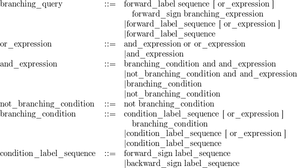
In branching queries, a condition on a node with a given label holds if there exists a label sequence that fits to the condition. For example, the root//  /
/  [
[ 
 //
//  and not
 /
/  ]/
]/  query seeks nodes with label
  such that the node can be reached from the root in such a way that the labels of the last two nodes are
  and
and  , furthermore, there exists a parent of the node with label
  whose label is
  , and among the descendants of the node with label
  there is one with label
  , but it has no children with label
  that has a parent with label
  .
.
If we omit all conditions written between signs [ ] from a branching query, then we get the main query corresponding to the branching query. In our previous example, this is the query root//  /
/  /
/  . The main query always corresponds to a forward label sequence.
A directed graph can be assigned naturally to branching queries. Assign nodes with the same label to the label sequence of the query, in case of separators / and  , connect the successive nodes with a directed edge according to the separator, and in case of separators // and
  , draw the directed edge and label it with label // or
  . Finally, the logic connectives are assigned to the starting edge of the corresponding condition as a label. Thus, it might happen that an edge has two labels, for example // and “and”. Note that the graph obtained cannot contain a directed cycle because of the definition of the grammar.
A simple degree of complexity of the query can be defined using the tree obtained. Assign  to the nodes of the main query and to the nodes from which there is a directed path to a node of the main query. Then assign
  to the nodes that can be reached from the nodes with sign
  on a directed path and have no sign yet. Assign
  to the nodes from which a node with sign
  can be reached and have no sign yet. Assign
  to the nodes that can be reached from nodes with sign
  and have no sign yet, etc. Assign
  to the nodes that can be reached from nodes with sign
  and have no sign yet, then assign
  to the nodes from which nodes with sign
  can be reached and have no sign yet. The value of the greatest sign in the query is called the depth of the tree. The depth of the tree shows how many times the direction changes during the evaluation of the query, that is, we have to seek children or parents according to the direction of the edges. The same query could have been given in different ways by composing the conditions differently, but it can be proved that the value defined above does not depend on that, that is why the complexity of a query was not defined as the number of conditions composed.
The 1-index assigns the nodes into classes according to incoming paths, using bisimulations. The concept of stability used for computations was descendant-stability. A set  of the nodes of a graph is descendant-stable with respect to a set
  of nodes if
  or
or  , where
  is the set of nodes that can be reached by edges from
  . A partition is stable if any two elements of the partition are descendant-stable with respect to each other. The 1-index is the coarsest descendant-stable partition that assigns nodes with the same label to same classes, which can be computed using the
 PT-algorithm. In case of branching queries, we also have to go backwards on directed edges, so we will need the concept of ancestor-stability as well. A set  of nodes of a graph is ancestor-stable with respect to a set
  of the nodes if
  or
or  , where
  denotes the nodes from which a node of
  can be reached.
Definition 20.41 The FB-index is the coarsest refinement of the basic partition that is ancestor-stable and descendant-stable.
Note that if the direction of the edges of the graph is reversed, then an ancestor-stable partition becomes a descendant-stable partition and vice versa, therefore the PT-algorithm and its improvements can be used to compute the coarsest ancestor-stable partition. We will use this in the following algorithm. We start with classes of nodes with the same label, compute the 1-index corresponding to this partition, then reverse the direction of the edges, and refine this by computing the 1-index corresponding to this. When the algorithm stops, we get a refinement of the initial partition that is ancestor-stable and descendant-stable at the same time. This way we obtain the coarsest such partition. The proof of this is left to the Reader.
FB-Index-Creator(
)
1
Start with classes of nodes with the same label. 2
WHILEchanges 3
DO
Compute the 1-index. 4
Reverse the direction
of edges, and compute the 1-index. 5
RETURN
The following corollary follows simply from the two stabilities.
Corollary 20.42 The FB-index is safe and exact with respect to branching queries.
The complexity of the algorithm can be computed from the complexity of the PT-algorithm. Since  is always the refinement of the previous partition, in the worst case refinement is done one by one, that is, we always take one element of a class and create a new class consisting of that element. So in the worst case, the cycle is repeated
  times. Therefore, the cost of the algorithm is at most
  .
.
The partition gained by executing the cycle only once is called the F+B-index, the partition obtained by repeating the cycle twice is the F+B+F+B-index, etc.
The following proposition can be proved easily.
Claim 20.43 The F+B+F+B+  +F+B-index, where F+B appears
  times, is safe and exact with respect to the branching queries of depth at most
  .
.
Nodes of the same class according to the FB-index cannot be distinguished by branching queries. This restriction is usually too strong, therefore the size of the FB-index is usually much smaller than the size of the original graph. Very long branching queries are seldom used in practice, so we only require local equivalence, similarly to the A( )-index, but now we will describe it with two parameters depending on what we want to restrict: the length of the directed paths or the length of the paths with reversed direction. We can also restrict the depth of the query. We can introduce the FB(
 )-index, with which such restricted branching queries can be evaluated exactly. We can also evaluate branching queries that do not satisfy the restrictions, but then the result must be checked.
FB(
)-Index-Creator(
)
1
start with classes of nodes with the same label. 2
FOR
TO3
DONaive-Approximation()Compute the A(
)-index. 4
Naive-Approximation()Reverse the direction
of the edges, and compute the A(
)-index. 5
RETURN


The cost of the algorithm, based on the computation cost of the A( )-index, is at most
  , which is much better than the computation cost of the FB-index, and the index graph obtained is also usually much smaller.
The following proposition obviously holds for the index obtained.
Claim 20.44 The FB( )-index is safe and exact for the branching queries in which the length of forward-sequences is at most
  , the length of backward-sequences is at most
  , and the depth of the tree corresponding to the query is at most
  .
.
As a special case we get that the FB( )-index is the FB-index, the FB(
 )-index is the F+B+
  +F+B-index, where F+B appears
  times, the FB(
 )-index is the 1-index, and the FB(
 )-index is the A(
 )-index.
Exercises
20.7-1 Prove that the algorithm FB-Index-Creator produces the coarsest ancestor-stable and descendant-stable refinement of the basic partition.
20.7-2 Prove Proposition 20.44.
In database management we usually have three important aspects in mind. We want space requirement to be as small as possible, queries to be as fast as possible, and insertion, deletion and modification of the database to be as quick as possible. Generally, a result that is good with respect to one of these aspects is worse with respect to another aspect. By adding indexes of typical queries to the database, space requirement increases, but in return we can evaluate queries on indexes which makes them faster. In case of dynamic databases that are often modified we have to keep in mind that not only the original data but also the index has to be modified accordingly. The most costly method which is trivially exact is that we create the index again after every modification to the database. It is worth seeking procedures to get the modified indexes by smaller modifications to those indexes we already have.
Sometimes we index the index or its modification as well. The index of an index is also an index of the original graph, although formally it consists of classes of index nodes, but we can unite the elements of the index nodes belonging to the same class. It is easy to see that by that we get a partition of the nodes of the graph, that is, an index.
In the following, we will discuss those modifications of semi-structured databases when a new graph is attached to the root and when a new edges is added to the graph, since these are the ones we need when creating a new website or a new reference.
Suppose that  is the 1-index of graph
  . Let
. Let  be a graph that has no common node with
  . Denote by
  the 1-index of
  . Let
. Let  be the graph obtained by uniting the roots of
  and
and  . We want to create
  using
using  and
and  . The following proposition will help us.
Claim 20.45 Let  be the 1-index of graph
  , and let
  be an arbitrary refinement of
  . Then
  .
.
Proof. Let  and
and  be two nodes of
  . We have to show that
  and
and  are bisimilar in
  with respect to the 1-index if and only if
  and
and  are bisimilar in the index graph
  with respect to the 1-index of
  . Let
. Let  and
and  be bisimilar in
  with respect to the 1-index. We will prove that there is a bisimulation according to which
  and
and  are bisimilar in
  . Since the 1-index is the partition corresponding to the coarsest bisimulation, the given bisimulation is a refinement of the bisimulation corresponding to the 1-index, so
  and
and  are also bisimilar with respect to the bisimulation corresponding to the 1-index of
  . Let
. Let  if and only if
  and
and  are bisimilar in
  with respect to the 1-index. Note that since
  is a refinement of
  , all elements of
  and
and  are bisimilar in
  if
if  . To show that the relation
  is a bisimulation, let
  be a parent of
  , where
  is a parent of
  , and
, and  is an element of
  . Then
  ,
,  and
and  are bisimilar in
  , so there is a parent
  of
of  for which
  and
and  are bisimilar in
  . Therefore
  is a parent of
  , and
, and  . Since bisimulation is symmetric, relation
  is also symmetric. We have proved the first part of the proposition.
Let  and
and  be bisimilar in
  with respect to the 1-index of
  . It is sufficient to show that there is a bisimulation on the nodes of
  according to which
  and
and  are bisimilar. Let
  if and only if
  with respect to the 1-index of
  . To prove bisimilarity, let
  be a parent of
  . Then
  is also a parent of
  . Since
  and
and  are bisimilar if
  , there is a parent
  of
of  for which
  and
and  are bisimilar with respect to the 1-index of
  , and
, and  is a parent of an element
  of
of  . Since
  and
and  are bisimilar, there is a parent
  of
of  such that
  and
and  are bisimilar. Using the first part of the proof, it follows that
  and
and  are bisimilar with respect to the 1-index of
  . Since bisimilarity is transitive,
  and
and  are bisimilar with respect to the 1-index of
  , so
, so  . Since relation
  is symmetric by definition, we get a bisimulation.
As a consequence of this proposition,  can be created with the following algorithm for disjoint
  and
and  .
.
Graphaddition-1-Index(
)
  1          is the basic partition according to labels.
  2          is the basic partition according to labels.
  3          is the 1-index of .
  4          is the 1-index of .
  5         The 1-indexes are joined at the roots.
  6          is the basic partition according to labels.
  7          is the 1-index of .
  8  RETURN
To compute the cost of the algorithm, suppose that the 1-index  of
of  is given. Then the cost of the creation of
  is
is  , where
  and
and  denote the number of nodes and edges of the graph, respectively.
To prove that the algorithm works, we only have to notice that  is a refinement of
  if
if  and
and  are disjoint. This also implies that index
  is safe and exact, so we can use this as well if we do not want to find the minimal index. This is especially useful if new graphs are added to our graph many times. In this case we use the lazy method, that is, instead of computing the minimal index for every pair, we simply sum the indexes of the addends and then minimize only once.
Claim 20.46 Let  be the 1-index of graph
  ,
,  , and let the graphs be disjoint. Then
  for the 1-index
  of the union of the graphs joined at the roots.
In the following we will examine what happens to the index if a new edge is added to the graph. Even an operation like this can have significant effects. It is not difficult to construct a graph that contains two identical subgraphs at a distant of 2 from the root which cannot be contracted because of a missing edge. If we add this critical edge to the graph, then the two subgraphs can be contracted, and therefore the size of the index graph decreases to about the half of its original size.
Suppose we added a new edge to graph  from
from  to
to  . Denote the new graph by
  , that is,
  . Let partition
  be the 1-index of
  . If there was an edge from
  to
to  in
in  , then the index graph does not have to be modified, since there is a parent of the elements of
  , that is, of all elements bisimilar to
  , in
, in  whose elements are bisimilar to
  . Therefore
  .
.
If there was no edge from  to
to  , then we have to add this edge, but this might cause that
  will no longer be stable with respect to
  . Let
. Let  be the partition we get from
  by splitting
  in such a way that
  is in one part and the other elements of
  are in the other, and leaving all other classes of the partition unchanged.
  defines its edges the usual way, that is, if there is an edge from an element of a class to an element of another class, then we connect the two classes with an edge directed the same way.
Let partition  be the original
  . Then
  is a refinement of
  , and
, and  is stable with respect to
  according to
  . Note that the same invariant property appeared in the
 PT-algorithm for partitions  and
and  . Using Proposition 20.45 it is enough to find a refinement of
  . If we can find an arbitrary stable refinement of the basic partition of
  , then, since the 1-index is the coarsest stable partition, this will be a refinement of
  .
.  is a refinement of the basic partition, that is, the partition according to labels, and so is
  . So if
  is stable, then we are done. If it is not, then we can stabilize it using the
 PT-algorithm by starting with the above partitions  and
and  . First we have to examine those classes of the partition that contain a children of
  , because these might lost their stability with respect to the two new classes gained by the split. The
 PT-algorithm stabilizes these by splitting them, but because of this we now have to check their children, since they might have lost stability because of the split, etc. We can obtain a stable refinement using this stability-propagator method. Since we only walk through the nodes that can be reached from  , this might not be the coarsest stable refinement. We have shown that the following algorithm computes the 1-index of the graph
  .
.
Edgeaddition-1-Index(
)
1

is the basic partition according to labels. 2

is the 1-index of
. 3

Add edge
. 4
IF
If there was an edge from
to
, then no modification is needed. 5
THENRETURN6

Split
. 7
8


is the old partition. 9

Add an edge from
to
. 10

Replace
with
and
. 11

Determine the edges of
. 12

Execute the
PT-algorithmstarting with
and
. 13

is the coarsest stable refinement. 14
RETURN
Step 13 can be omitted in practice, since the stable refinement obtained in step 12 is a good enough approximation of the coarsest stable partition, there is only 5% difference between them in size.
In the following we will discuss how FB-indexes and A( )-indexes can be refreshed. The difference between FB-indexes and 1-indexes is that in the FB-index, two nodes are in the same similarity class if not only the incoming but also the outgoing paths have the same label sequences. We saw that in order to create the FB-index we have to execute the
 PT-algorithm twice, using it on the graph with the edges reversed at the second time. The FB-index can be refreshed similarly to the 1-index. The following proposition can be proved similarly to Proposition 20.45, therefore we leave it to the Reader.
Claim 20.47 Let  be the FB-index of graph
  , and let
  be an arbitrary refinement of
  . Denote by
  the FB-index of
  . Then
  .
.
As a consequence of the above proposition, the FB-index of  can be created using the following algorithm for disjoint
  and
and  .
.
Graphaddition-FB-Index(
)
1FB-Index-Creator()
is the FB-index of
. 2
FB-Index-Creator()
is the FB-index of
. 3

Join the FB-indexes at their roots. 4
FB-Index-Creator()
is the FB-index of
. 5
RETURN


When adding edge  , we must keep in mind that stability can be lost in both directions, so not only
  but also
  has to be split into
  ,
,  and
and  ,
,  , respectively. Let
  be the partition before the modification, and
  the partition obtained after the splits. We start the
 PT-algorithm with  and
and  in step 3 of the algorithm
 FB-Index-Creator. When stabilizing, we will now walk through all descendants of  and all ancestors of
  .
.
Edgeaddition-FB-Index(
)
1FB-index-creator()
is the FB-index of
. 2
Add edge
. 3
IF
If there was an edge from
to
, then no modification is needed. 4
THENRETURN5

Split
. 6
7

Split
. 8
9


is the old partition. 10

Add an edge form
to
. 11

Replace
with
and
,
with
and
. 12

Determine the edges of
. 13
FB-Index-Creator()Start the
PT-algorithmwith
and
in the algorithm
FB-Index-Creator. 14FB-Index-Creator()
is the coarsest ancestor-stable and descendant-stable refinement. 15
RETURN


Refreshing the A( )-index after adding an edge is different than what we have seen. There is no problem with adding a graph though, since the following proposition holds, the proof of which is left to the Reader.
Claim 20.48 Let  be the A(
 )-index of graph
  , and let
  be an arbitrary refinement of
  . Denote by
  the A(
 )-index of
  . Then
  .
.
As a consequence of the above proposition, the A( )-index of
  can be created using the following algorithm for disjoint
  and
and  .
.
Graphaddition-A(
)-Index(
)
1

is the basic partition according to labels. 2
Naive-Approximation()
is the A(
)-index of
. 3


is the basic partition according to labels. 4
Naive-Approximation()
is the A(
)-index of
. 5

Join the A(
)-indexes. 6


is the basic partition according to labels. 7
Naive-Approximation()
is the A(
)-index of
. 8
RETURN


If we add a new edge  to the graph, then, as earlier, first we split
  into two parts, one of which is
  , then we have to repair the lost
  -stabilities walking through the descendants of
  , but only within a distant of
  . What causes the problem is that the A(
 )-index contains information only about
  -bisimilarity, it tells us nothing about
  -bisimilarity. For example, let
  be a child of
  , and let
  . When stabilizing according to the 1-index,
  has to be detached from its class if there is an element in this class that is not a children of
  . This condition is too strong in case of the A(1)-index, and therefore it causes too many unnecessary splits. In this case,
  should only be detached if there is an element in its class that has no 0-bisimilar parent, that is, that has the same label as
  . Because of this, if we refreshed the A(
 )-index the above way when adding a new edge, we would get a very bad approximation of the A(
 )-index belonging to the modification, so we use a different method. The main idea is to store all A(
 )-indexes not only the A(
 )-index, where
  . Yi et al. give an algorithm based on this idea, and creates the A(
 )-index belonging to the modification. The given algorithms can also be used for the deletion of edges with minor modifications, in case of 1-indexes and A(
 )-indexes.
Exercises
20.8-1 Prove Proposition 20.47.
20.8-2 Give an algorithm for the modification of the index when an edge is deleted from the data graph. Examine different indexes. What is the cost of the algorithm?
20.8-3 Give algorithms for the modification of the D( )-index when the data graph is modified.
PROBLEMS |
20-1 Implication problem regarding constraints
Let  and
and  be regular expressions,
  and
and  two nodes. Let predicate
  mean that
  can be reached from
  by a label sequence that fits to
  . Denote by
  the constraint
  .
.  if
if  and
and  . Let
. Let  be a finite set of constraints, and
  a constraint.
-
a. Prove that the implication problem
 is a 2-EXPSPACE problem.
 -
b. Denote by
 the constraint
  . Prove that the implication problem is undecidable with respect to this class.
20-2 Transformational distance of trees
Let the transformational distance of vertex-labeled trees be the minimal number of basic operations with which a tree can be transformed to the other. We can use three basic operations: addition of a new node, deletion of a node, and renaming of a label.
-
a. Prove that the transformational distance of trees
 and
and  can be computed in
  time, with storage cost of
  , where
  is the number of nodes of the tree and
  is the depth of the tree.
 -
b. Let
 and
and  be two trees. Give an algorithm that generates all pairs
  , where
  and
and  simulates graphs
  and
and  , respectively, and the transformational distance of
  and
and  is less then a given integer
  . (This operation is called approximate join.)
20-3 Queries of distributed databases
A distributed database is a vertex-labeled directed graph the nodes of which are distributed in  partitions (servers). The edges between different partitions are cross references. Communication is by message broadcasting between the servers. An algorithm that evaluates a query is efficient, if the number of communication steps is constant, that is, it does not depend on the data and the query, and the size of the data transmitted during communication only depends on the size of the result of the query and the number of cross references. Prove that an efficient algorithm can be given for the regular query of distributed databases in which the number of communication steps is 4, and the size of data transmitted is
  , where
  is the size of the result of the query, and
  is the number of cross references. (Hint. Try to modify the algorithm
 Naive-Evaluation for this purpose.)
CHAPTER NOTES |
This chapter examined those fields of the world of semi-structured databases where the morphisms of graphs could be used. Thus we discussed the creation of schemas and indexes from the algorithmic point of view. The world of semi-structured databases and XML is much broader than that. A short summary of the development, current issues and the possible future development of semi-structured databases can be found in the paper of Vianu [336].
The paper of M. Henzinger, T. Henzinger and Kopke [162] discusses the computation of the maximal simulation. They extend the concept of simulation to infinite graphs that can be represented efficiently (these are called effective graphs), and prove that for such graphs, it can be determined whether two nodes are similar. In their paper, Corneil and Gotlieb [74] deal with quotient graphs and the determination of isomorphism of graphs. Arenas and Libkin [18] extend normal forms used in the relational model to XML documents. They show that arbitrary DTD can be rewritten without loss as XNF, a normal form they introduced.
Buneman, Fernandez and Suciu [50] introduce a query language, the UnQL, based on structural recursion, where the data model used is defined by bisimulation. Gottlob, Koch and Pichler [139] examine the classes of the query language XPath with respect to complexity and parallelization. For an overview of complexity problems we recommend the classical work of Garey and Johnson [128] and the paper of Stockmeyer and Meyer [308].
The PT-algorithm was first published in the paper of Paige and Tarjan [265]. The 1-index based on bisimulations is discussed in detail by Milo and Suciu [247], where they also introduce the 2-index, and as a generalization of this, the T-index.
The A( )-index was introduced by Kaushik, Shenoy, Bohannon and Gudes [193]. The D(
 )-index first appeared in the work of Chen, Lim and Ong [63]. The M(
 )-index and the M
  -index, based on frequent queries, are the results of He and Yang [159]. FB-indexes of branching queries were first examined by Kaushik, Bohannon, Naughton and Korth [191]. The algorithms of the modifications of 1-indexes, FB-indexes and A(
 )-indexes were summarized by Kaushik, Bohannon, Naughton and Shenoy [192]. The methods discussed here are improved and generalized in the work of Yi, He, Stanoi and Yang [352]. Polyzotis and Garafalakis use a probability model for the study of the selectivity of queries [275]. Kaushik, Krishnamurthy, Naughton and Ramakrishnan [194] suggest the combined use of structural indexes and inverted lists.
The book of Tucker [325] and the encyclopedia edited by Khosrow-Pour [198] deal with the use of XML in practice.
Table of Contents
- 9. Bioinformatics
- 21.1 Algorithms on sequences
- 21.1.1 Distances of two sequences using linear gap penalty
- 21.1.2 Dynamic programming with arbitrary gap function
- 21.1.3 Gotoh algorithm for affine gap penalty
- 21.1.4 Concave gap penalty
- 21.1.5 Similarity of two sequences, the Smith-Waterman algorithm
- 21.1.6 Multiple sequence alignment
- 21.1.7 Memory-reduction with the Hirschberg algorithm
- 21.1.8 Memory-reduction with corner-cutting
- 21.2 Algorithms on trees
- 21.3 Algorithms on stochastic grammars
- 21.4 Comparing structures
- 21.5 Distance based algorithms for constructing evolutionary trees
- 21.6 Miscellaneous topics
- 10. Computer Graphics
- 11. Human-Computer Interaction
Table of Contents
- 21.1 Algorithms on sequences
- 21.1.1 Distances of two sequences using linear gap penalty
- 21.1.2 Dynamic programming with arbitrary gap function
- 21.1.3 Gotoh algorithm for affine gap penalty
- 21.1.4 Concave gap penalty
- 21.1.5 Similarity of two sequences, the Smith-Waterman algorithm
- 21.1.6 Multiple sequence alignment
- 21.1.7 Memory-reduction with the Hirschberg algorithm
- 21.1.8 Memory-reduction with corner-cutting
- 21.2 Algorithms on trees
- 21.3 Algorithms on stochastic grammars
- 21.4 Comparing structures
- 21.5 Distance based algorithms for constructing evolutionary trees
- 21.6 Miscellaneous topics
In this chapter at first we present algorithms on sequences, trees and stochastic grammars, then we continue with algorithms of comparison of structures and constructing of evolutionary trees, and finish the chapter with some rarely discussed topics of bioinformatics.
In this section, we are going to introduce dynamic programming algorithms working on sequences. Sequences are finite series of characters over a finite alphabet. The basic idea of dynamic programming is that calculations for long sequences can be given via calculations on substrings of the longer sequences.
The algorithms introduced here are the most important ones in bioinformatics, they are the basis of several software packages.
DNA contains the information of living cells. Before the duplication of cells, the DNA molecules are doubled, and both daughter cells contain one copy of DNA. The replication of DNA is not perfect, the stored information can be changed by random mutations. Random mutations creates variants in the population, and these variants evolve to new species.
Given two sequences, we can ask the question how much the two species are related, and how many mutations are needed to describe the evolutionary history of the two sequences.
We suppose that mutations are independent from each other, and hence, the probability of a series of mutations is the product of probabilities of the mutations. Each mutation is associated with a weight, mutations with high probability get a smaller weight, mutations with low probability get a greater weight. A reasonable choice might be the logarithm of one over the probability of the mutation. In this case the weight of a series of mutations is the sum of the weights of the individual mutations. We also assume that mutation and its reverse have the same probability, therefore we study how a sequence can be transfered into another instead of evolving two sequences from a common ancestor. Assuming minimum evolution minimum evolution, we are seeking for the minimum weight series of mutations that transforms one sequence into another. An important question is how we can quickly find such a minimum weight series. The naive algorithm finds all the possible series of mutations and chooses the minimum weight. Since the possible number of series of mutations grows exponentially – as we are going to show it in this chapter –, the naive algorithm is obviously too slow.
We are going to introduce the Sellers' algorithm [299]. Let  be a finite set of symbols, and let
  denote the set of finite long sequences over
  . The
. The  long prefix of
  will be denoted by
  , and
, and  denotes the
  th character of
  . The following transformations can be applied for a sequence:
-
Insertion of symbol
 before position
  , denoted by
  .
. -
Deletion of symbol
 at position
  , denoted by
  .
. -
Substitution of symbol
 to symbol
  at position
  , denoted by
  .
.
The concatenation of mutations is denoted by the  symbol.
  denotes the set of finite long concatenations of the above mutations, and
  denotes that
  transforms a sequence
  into sequence
  . Let
. Let  a weight function such that for any
  ,
,  and
and  transformations satisfying

the

equation also holds. Furthermore, let  be independent from
  . The transformation distance between two sequences,
  and
and  , is the minimum weight of transformations transforming
  into
into  :
:

If we assume that  satisfies


for any  ,
,  ,
,  , then the
  transformation distance is indeed a metric on
  .
.
Since  is a metric, it is enough to concern with transformations that change each position of a sequence at most once. Series of transformations are depicted with sequence alignments. By convention, the sequence at the top is the ancestor and the sequence at the bottom is its descendant. For example, the alignment below shows that there were substitutions at positions three and five, there was an insertion in the first position and a deletion in the eighth position.
- A U C G U A C A G |
U A G C A U A - A G |
A pair at a position is called aligned pair. The weight of the series of transformations described by the alignment is the sum of the weights of aligned pairs. Each series of mutations can be described by an alignment, and this description is unique up the permutation of mutations in the series. Since the summation is commutative, the weight of the series of mutations does not depend on the order of mutations.
We are going to show that the number of possible alignments also grows exponentially with the length of the sequences. The alignments that do not contain this pattern
# - |
- # |
where # an arbitrary character of  gives a subset of possible alignments. The size of this subset is
  , since there is a bijection between this set of alignments and the set of coloured sequences that contains the characters of
  and
and  in increasing order, and the characters of
  is coloured with one colour, and the characters of
  is coloured with the other colour. For example, if
  , then
  .
.
An alignment whose weight is minimal called an optimal alignment. Let the set of optimal alignments of  and
and  be denoted by
  , and let
  denote the weights of any alignment in
  .
.
The key of the fast algorithm for finding an optimal alignment is that if we know  ,
,  , and
, and  , then we can calculate
  in constant time. Indeed, if we delete the last aligned pair of an optimal alignment of
  and
and  , we get the optimal alignment of
  and
and  , or
, or  and
and  or
or  and
and  , depending on the last aligned column depicts a deletion, an insertion, substitution or match, respectively. Hence,
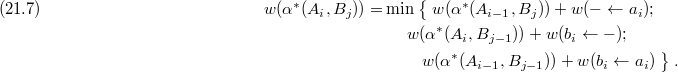
The weights of optimal alignments are calculated in the so-called dynamic programming table,  . The
. The  element of
  contains
  . Comparing of an
  and an
  long sequence requires the fill-in of an
  table, indexing of rows and columns run from
  till
till  and
and  , respectively. The initial conditions for column
  and row
  are
are


The table can be filled in using Equation (21.7). The time requirement for the fill-in is  . After filling in the dynamic programming table, the set of all optimal alignments can be find in the following way, called trace-back. We go from the right bottom corner to the left top corner choosing the cell(s) giving the optimal value of the current cell (there might be more than one such cells). Stepping up from position
  means a deletion, stepping to the left means an insertion, and the diagonal steps mean either a substitution or a match depending on whether or not
  . Each step is represented with an oriented edge, in this way, we get an oriented graph, whose vertices are a subset of the cells of the dynamic programming table. The number of optimal alignments might grow exponentially with the length of the sequences, however, the set of optimal alignments can be represented in polynomial time and space. Indeed, each path from
  to
to  on the oriented graph obtained in the trace-back gives an optimal alignment.
Since deletions and insertions get the same weight, the common name of them is indel or gap, and their weights are called gap penalty. Usually gap penalties do not depend on the deleted or inserted characters. The gap penalties used in the previous section grow linearly with the length of the gap. This means that a long indel is considered as the result of independent insertions or deletions of characters. However, the biological observation is that long indels can be formed in one evolutionary step, and these long indels are penalised too much with the linear gap penalty function. This observation motivated the introduction of more complex gap penalty functions [339]. The algorithm introduced by Waterman et al. penalises a  long gap with
  . For example the weight of this alignment:
- - A U C G A C G U A C A G |
U A G U C - - - A U A G A G |
is  .
.
We are still seeking for the minimal weight series of transformations transforming one sequence into another or equivalently for an optimal alignment. Since there might be a long indel at the end of the optimal alignment, above knowing  , we must know all
  ,
,  and
and  ,
,  to calculate
  . The dynamic programming recursion is given by the following equations:
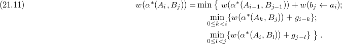
The initial conditions are:


The time requirement for calculating  is
is  , hence the running time of the fill-in part to calculate the weight of an optimal alignment is
 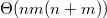 . Similarly to the previous algorithm, the set of optimal alignments represented by paths from
  to
to  can be found in the trace-back part.
If  , then the running time of this algorithm is
  . With restrictions on the gap penalty function, the running time can be decreased. We are going to show two such algorithms in the next two sections.
A gap penalty function is affine if

There exists a  running time algorithm for affine gap penalty [138]. Recall that in the Waterman algorithm,

where


The key of the Gotoh algorithm is the following reindexing
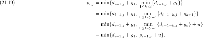
And similarly

In this way,  és
és  can be calculated in constant time, hence
  . Thus, the running time of the algorithm remains
  , and the algorithm will be only a constant factor slower than the dynamic programming algorithm for linear gap penalties.
There is no biological justification for the affine gap penalty function [36], [137], its wide-spread use (for example, CLUSTAL-W [322]) is due to its low running time. There is a more realistic gap penalty function for which an algorithm exists whose running time is slightly more than the running time for affine gap penalty, but it is still significantly better than the cubic running time algorithm of Waterman et al. [124], [246].
A gap penalty function is concave if for each  ,
,  . Namely, the increasement of gap extensions are penalised less and less. It might happen that the function starts decreasing after a given point, to avoid this, it is usually assumed that the function increases monotonously. Based on empirical data [36], if two sequences evolved for
  PAM unit [80], the weight of a
  long indel is

which is also a concave function. (One PAM unit is the time span on which 1% of the sequence changed.) There exist an 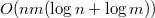 running time algorithm for concave gap penalty functions. this is a so-called forward looking algorithm. The
 Forward-Looking algorithm calculates the  th row of the dynamic programming table in the following way for an arbitrary gap penalty function:
Forward-Looking
1FOR2
3
4
FOR5
6
7
At this step, we suppose that
and
are already calculated. 8
FOR
Inner cycle. 9
IF
THEN1011

where  is the gap penalty function and
  is a pointer whose role will be described later. In row
  , we assume that we already calculated
  and
and  . It is easy to show that the forward looking algorithm makes the same comparisons as the traditional, backward looking algorithm, but in a different order. While the backward looking algorithm calculates
  at the
  th position of the row looking back to the already calculated entries of the dynamic programming table, the
 Forward-Looking algorithm has already calculated  by arriving to the
  th position of the row. On the other hand, it sends forward candidate values for
  ,
,  , and by arriving to cell
  , all the needed comparisons of candidate values have been made. Therefore, the
 Forward-Looking algorithm is not faster than the traditional backward looking algorithm, however, the conception helps accelerate the algorithm.
The key idea is the following.
Lemma 21.1 Let  be the actual cell in the row. If

then for all 

Proof. From the condition it follows that there is a  for which

Let us add  to the equation:

For each concave gap penalty function,

rearranging this and using Equation (21.25)

The idea of the algorithm is to find the position with a binary search from where the actual cell cannot send forward optimal  values. This is still not enough for the desired acceleration since
  number of candidate values should be rewritten in the worst case. However, the corollary of the previous lemma leads to the desired acceleration:
Corollary 21.2 Before the  th cell sends forward candidate values in the inner cycle of the forward looking algorithm, the cells after cell
  form blocks, each block having the same pointer, and the pointer values are decreasing by blocks from left to right.
The pseudocode of the algorithm is the following:
Forward-Looking-Binary-Searching(
)
1;
;
2
FOR
TO3
DO4
5
At this step, we suppose that
and
are already calculated. 6
IF
THEN7THEN8
IF
AND9
THEN;
10
ELSE IF11
THEN
12
IF13
THEN;
14
ELSE15
IF16
THEN17
ELSE18
19
20

The algorithm works in the following way: for each row, we maintain a variable storing the number of blocks, a list of positions of block ends, and a list of pointers for each block. For each cell  , the algorithm finds the last position for which the cell gives an optimal value using binary search. There is first a binary search for the blocks then for the positions inside the choosen block. It is enough to rewrite three values after the binary searches: the number of blocks, the end of the last block and its pointer. Therefore the most time consuming part is the binary search, which takes
  time for each cell.
We do the same for columns. If the dynamic programming table is filled in row by row, then for each position  in row
  , the algorithms uses the block system of column
  . Therefore the running time of the algorithm is
  .
.
We can measure not only the distance but also the similarity of two sequences. For measuring the similarity of two characters,  , the most frequently used function is the log-odds:

where  is the joint probability of the two characters (namely, the probability of observing them together in an alignment column),
  and
and  are the marginal probabilities. The similarity is positive if
  , otherwise negative. Similarities are obtained from empirical data, for aminoacids, the most commonly used similarities are given by the PAM and BLOSUM matrices.
If we penalise gaps with negative numbers then the above described, global alignment algorithms work with similarities by changing minimalisation to maximalisation.
It is possible to define a special problem that works for similarities and does not work for distances. It is the local similarity problem or the local sequence alignment problem [305]. Given two sequences, a similarity and a gap penalty function, the problem is to give two substrings of the sequences whose similarity is maximal. A substring of a sequence is a consecutive part of the sequence. The biological motivation of the problem is that some parts of the biological sequences evolve slowly while other parts evolve fast. The local alignment finds the most conservated part of the two sequences. Local alignment is widely used for homology searching in databases. The reason why local alignments works well for homology searching is that the local alignment score can separate homologue and non-homologue sequences better since the statistics is not decreased due to the variable regions of the sequences.
The Smith-Waterman algorithm work in the following way. The initial conditions are:

Considering linear gap penalty, the dynamic programming table is filled in using the following recursions:

Here  , the gap penalty is a negative number. The best local similarity score of the two sequences is the maximal number in the table. The trace-back starts in the cell having the maximal number, and ends when first reaches a
  .
.
It is easy to prove that the alignment obtained in the trace-back will be locally optimal: if the alignment could be extended at the end with a sub-alignment whose similarity is positive then there would be a greater number in the dynamic programming table. If the alignment could be extended at the beginning with a subalignment having positive similarity then the value at the end of the traceback would not be  .
.
The multiple sequence alignment problem was introduced by David Sankoff [294], and by today, the multiple sequence alignment has been the central problem in bioinformatics. Dan Gusfield calls it the Holy Grail of bioinformatics [148]. Multiple alignments are widespread both in searching databases and inferring evolutionary relationships. Using multiple alignments, it is possible to find the conservated parts of a sequence family, the positions that describe the functional properties of the sequence family. AS Arthur Lesk said: [169]: What two sequences whisper, a multiple sequence alignment shout out loud.
The columns of a multiple alignment of  sequences is called aligned
  -tuples. The dynamic programming for the optimal multiple alignment is the generalisation of the dynamic programming for optimal pairwise alignment. To align
  sequences, we have to fill in a
  dimensional dynamic programming table. To calculate an entry in this table using linear gap penalty, we have to look back to a
  dimensional hypercube. Therefore, the memory requirement in case of
  sequence,
  long each is
  , and the running time of the algorithm is
  if we use linear gap penalty, and
  with arbitrary gap penalty.
There are two fundamental problems with the multiple sequence alignment. The first is an algorithmic problem: it is proven that the multiple sequence alignment problem is NP-complete [337]. The other problem is methodical: it is not clear how to score a multiple alignment. An objective scoring function could be given only if the evolutionary relationships were known, in this case an aligned  -tuple could be scored according to an evolutionary tree [264].
A heuristic solution for both problems is the iterative sequence alignment [105], [75], [322]. This method first construct a guide-tree using pairwise distances (such tree-building methods are described in section 21.5). The guide-tree is used then to construct a multiple alignment. Each leaf is labelled with a sequence, and first the sequences in “cherry-motives” are aligned into each other, then sequence alignments are aligned to sequences and sequence alignments according to the guide-tree. The iterative sequence alignment method uses the “once a gap – always gap” rule. This means that gaps already placed into an alignment cannot be modified when aligning the alignment to other alignment or sequence. The only possibility is to insert all-gap columns into an alignment. The aligned sequences are usually described with a profile. The profile is a  table, where
  is the length of the alignment. A column of a profile contains the statistics of the corresponding aligned
  -tuple, the frequencies of characters and the gap symbol.
The obtained multiple alignment can be used for constructing another guide-tree, that can be used for another iterative sequence alignment, and this procedure can be iterated till convergence. The reason for the iterative alignment heuristic is that the optimal pairwise alignment of closely related sequences will be the same in the optimal multiple alignment. The drawback of the heuristic is that even if the previous assumption is true, there might be several optimal alignments for two sequences, and their number might grow exponentially with the length of the sequences. For example, let us consider the two optimal alignments of the sequences AUCGGUACAG and AUCAUACAG.

We cannot choose between the two alignments, however, in a multiple alignment, only one of them might be optimal. For example, if we align the sequence AUCGAU to the two optimal alignments, we get the following locally optimal alignments:
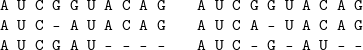
The left alignment is globally optimal, however, the right alignment is only locally optimal.
Hence, the iterative alignment method yields only a locally optimal alignment. Another problem of this method is that it does not give an upper bound for the goodness of the approximation. In spite of its drawback, the iterative alignment methods are the most widely used ones for multiple sequence alignments in practice, since it is fast and usually gives biologically reasonable alignments. Recently some approximation methods for multiple sequence alignment have been published with known upper bounds for their goodness [149], [283]. However, the bounds biologically are not reasonable, and in practice, these methods usually give worse results than the heuristic methods.
We must mention a novel greedy method that is not based on dynamic programming. The DiAlign [249], [250], [251] first searches for gap-free homologue substrings by pairwise sequence comparison. The gap-free alignments of the homologous substrings are called diagonals of the dynamic programming name, hence the name of the method: Diagonal Alignment. The diagonals are scored according to their similarity value and diagonals that are not compatible with high-score diagonals get a penalty. Two diagonals are not compatible if they cannot be in the same alignment. After scoring the diagonals, they are aligned together a multiple alignment in a greedy way. First the best diagonal is selected, then the best diagonal that is comparable with the first one, then the third best alignment that is comparable with the first two ones, etc. The multiple alignment is the union of the selected diagonals that might not cover all the characters in the sequence. Those characters that were not in any of the selected diagonals are marked as “non alignable”. The drawback of the method is that sometimes it introduces too many gaps due to not penalising the gaps at all. However, DiAlign has been one of the best heuristic alignment approach and is widely used in the bioinformatics community.
If we want to calculate only the distance or similarity between two sequences and we are not interested in an optimal alignment, then in case of linear or affine gap penalties, it is very easy to construct an algorithm that uses only linear memory. Indeed, note that the dynamic programming recursion needs only the previous row (in case of filling in the dynamic table by rows), and the algorithm does not need to store earlier rows. On the other hand, once the dynamic programming table has reached the last row and forgot the earlier rows, it is not possible to trace-back the optimal alignment. If the dynamic programming table is scrolled again and again in linear memory to trace-back the optimal alignment row by row then the running time grows up to  , where
  is the length of the sequences.
However, it is possible to design an algorithm that obtains an optimal alignment in  running time and uses only linear memory. This is the Hirschberg algorithm [165], which we are going to introduce for distance-based alignment with linear gap penalty.
We introduce the suffixes of a sequence, a suffix is a substring ending at the end of the sequence. Let  denote the suffix of
  starting with character
  .
.
The Hirschberg algorithm first does a dynamic programming algorithm for sequences  and
and  using liner memory as described above. Similarly, it does a dynamic programming algorithm for the reverse of the sequences
  and
and  .
.
Based on the two dynamic programming procedures, we know what is the score of the optimal alignment of  and an arbitrary prefix of
  , and similarly what is the score of the optimal alignment of
  and an arbitrary suffix of
  . From this we can tell what is the score of the optimal alignment of
  and
and  :
:

and from this calculation it must be clear that in the optimal alignment of  and
and  ,
,  is aligned with the prefix
  for which

is minimal.
Since we know the previous rows of the dynamic tables, we can tell if  and
and  is aligned with any characters of
  or these characters are deleted in the optimal alignment. Similarly, we can tell if any character of
  is inserted between
  and
and  .
.
In this way, we get at least two columns of the optimal alignment. Then we do the same for  and the remaining part of the prefix of
  , and for
  and the remaining part of the suffix of
  . In this way we get alignment columns at the quarter and the three fourths of sequence
  . In the next iteration, we do the same for the for pairs of sequences, etc., and we do the iteration till we get all the alignment columns of the optimal alignment.
Obviously, the memory requirement still only grows linearly with the length of the sequences. We show that the running time is still  , where
  and
and  are the lengths of the sequences. This comes from the fact that the running time of the first iteration is
  , the running time of the second iteration is
  , where
  is the position for which we get a minimum distance in Eqn. (21.31). Hence the total running time is:

The dynamic programming algorithm reaches the optimal alignment of two sequences with aligning longer and longer prefixes of the two sequences. The algorithm can be accelerated with excluding the bad alignments of prefixes that cannot yield an optimal alignment. Such alignments are given with the ordered paths going from the right top and the left bottom corners to  , hence the name of the technique.
Most of the corner-cutting algorithms use a test value. This test value is an upper bound of the evolutionary distance between the two sequences. Corner-cutting algorithms using a test value can obtain the optimal alignment of two sequences only if the test value is indeed smaller then the distance between the two sequences, otherwise the algorithm stops before reaching the right bottom corner or gives a non-optimal alignment. Therefore these algorithms are useful for searching for sequences similar to a given one and we are not interested in sequences that are farther from the query sequence than the test value.
We are going to introduce two algorithms. the Spouge algorithm [307], [306] is a generalisation of the Fickett [107] and the Ukkonnen algorithm [333], [332]. The other algorithm was given by Gusfield, and this algorithm is an example for a corner-cutting algorithm that reaches the right bottom corner even if the distance between the two sequence is greater than the test value, but in this case the calculated score is bigger than the test value, indicating that the obtained alignment is not necessary optimal.
The Spouge algorithm calculates only those  for which

where  is the test value,
  is the gap penalty,
  and
and  are the length of the sequences. The key observation of the algorithm is that any path going from
  to
to  will increase the score of the alignment at least by
  . Therefore is
  is smaller than the distance between the sequences, the Spouge algorithm obtains the optimal alignments, otherwise will stop before reaching the right bottom corner.
This algorithm is a generalisation of the Fickett algorithm and the Ukkonen algorithm. Those algorithms also use a test value, but the inequality in the Fickett algorithm is:

while the inequality in the Ukkonnen algorithm is:

Since in both cases, the left hand side of the inequalities are not greater than the left end side of the Spouge inequality, the Fickett and the Ukkonnen algorithms will calculate at least as much part of the dynamic programming table than the Spouge algorithm. Empirical results proved that the Spouge algorithm is significantly better [306]. The algorithm can be extended to affine and concave gap penalties, too.
The  -difference global alignment problem [148] asks the following question: Is there an alignment of the sequences whose weight is smaller than
  ? The algorithm answering the question has
  running time, where
  is the length of the longer sequence. The algorithm is based on the observation that any path from
  to
to  having at most score
  cannot contain a cell
  for which
  . Therefore the algorithm calculates only those
  cells for which
  and disregards the
  neighbours of the border elements for which
  . If there exists an alignment with a score smaller or equal than
  , then
  and
and  is indeed the distance of the two sequences. Otherwise
  , and
, and  is not necessary the score of the optimal alignment since there might be an alignment that leaves the band defined by the
  inequality and still has a smaller score then the best optimal alignment in the defined band.
The corner-cutting technique has been extended to multiple sequence alignments scored by the sum-of-pairs scoring scheme [57]. The sum-of-pairs score is:

where  is the
  th aligned
  -tuple
  is the distance function on
  ,
,  is the number of sequences,
  is the character of the multiple alignment in the
  th row and
  th column. The
  -suffix of sequence
  is
is  . Let
. Let  denote the distance of the optimal alignment of the
  -suffix and the
  -suffix of the
  th and the
  th sequences. The Carillo and Lipman algorithm calculates only the positions for which

where  is the test value. The goodness of the algorithm follows from the fact that the sum-of-pairs score of the optimal alignment of the not yet aligned suffixes cannot be smaller than the sum of the scores of the optimal pairwise alignments. This corner cutting method can align at most six moderately long sequences [223].
Exercises
21.1-1 Show that the number of possible alignments of an  and an
  long sequences is
21.1-2 Give a series of pairs of sequences and a scoring scheme such that the number of optimal alignments grows exponentially with the length of the sequences.
21.1-3 Give the Hirschberg algorithm for multiple alignments.
21.1-4 Give the Hirschberg algorithm for affine gap penalties.
21.1-5 Give the Smith-Waterman algorithm for affine gap penalties.
21.1-6 Give the Spouge algorithm for affine gap penalties.
21.1-7 Construct an example showing that the optimal multiple alignment of three sequences might contain a pairwise alignment that is only suboptimal.
Algorithms introduced in this section work on rooted trees. The dynamic programming is based on the reduction to rooted subtrees. As we will see, above obtaining optimal cases, we can calculate algebraic expressions in the same running time.
The (weighted) parsimony principle is to describe the changes of biological sequences with the minimum number (minimum weight) of mutations. We will concern only with substitutions, namely, the input sequences has the same length and the problem is to give the evolutionary relationships of sequences using only substitutions and the parsimony principle. We can define the large and the small parsimony problem. For the large parsimony problem, we do not know the topology of the evolutionary tree showing the evolutionary relationships of the sequences, hence the problem is to find both the best topology and an evolutionary history on the tree. The solution is not only locally but globally optimal. It has been proved that the large parsimony problem is NP-complete [119].
The small parsimony problem is to find the most parsimonious evolutionary history on a given tree topology. The solution for the small parsimony problem is only locally optimal, and there is no guarantee for global optimum.
Each position of the sequences is scored independently, therefore it is enough to find a solution for the case where there is only one character at each leaf of the tree. In this case, the evolutionary history can be described with labelling the internal nodes with characters. If two characters at neighbouring vertices are the same, then no mutation happened at the corresponding edge, otherwise one mutation happened. The naive algorithm investigates all possible labelings and selects the most parsimonious solution. Obviously, it is too slow, since the number of possible labelings grows exponentially with the internal nodes of the tree.
The dynamic programming is based on the reduction to smaller subtrees [294]. Here the definition of subtrees is the following: there is a natural partial ordering on the nodes in the rooted subtree such that the root is the greatest node and the leaves are minimal. A subtree is defined by a node, and the subtree contains this node and all nodes that are smaller than the given node. The given node is the root of the subtree. We suppose that for any  child of the node
  and any character
  we know the minimum number of mutations that are needed on the tree with root
  given that there is
  at node
  . Let
. Let  denote this number. Then

where  is the set of children of
  ,
,  is the alphabet, and
  is
is  if
if  and
and  otherwise.
The minimum number of mutations on the entire tree is  , where
  is the root of the tree. A most parsimonious labelling can be obtained with trace-backing the tree from the root to the leaves, writing to each nodes the character that minimises Eqn. 21.39. To do this, we have to store
  for all
  and
and  .
.
The running time of the algorithm is  for one character, where
  is the number of nodes of the tree, and
  for entire sequences, where
  is the length of the sequences.
The input of the Felsenstein algorithm [104] is a multiple alignment of DNA (or RNA or protein) sequences, an evolutionary tree topology and edge lengths, and a model that gives for each pair of characters,  and
and  and time
  , what is the probability that
  evolves to
  duting time
  . Let
. Let  denote this probability. The equilibrium probability distribution of the characters is denoted by
  . The question is what is the likelihood of the tree, namely, what is the probability of observing the sequences at the leaves given the evolutionary parameters consisting of the edge lengths and parameters of the substitution model.
We assume that each position evolves independently, hence the probability of an evolutionary process is the product of the evolutionary probabilities for each position. Therefore it is enough to show how to calculate the likelihood for a sequence position. We show this for an example tree that can be seen on Figure 21.1.  will denote the character at node
  and
and  is the length of edge
  . Since we do not know the characters at the internal nodes, we must sum the probabilities for all possible configurations:

If we consider the four character alphabet of DNA, the summation has  members, an in case of
  species, it would have
  , namely the computational time grows exponentially with the number of sequences. However, if we move the expressions not depending on the summation index out of the summation, then we get the following product:
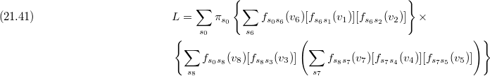
which can be calculated in significantly less time. Note that the parenthesis in (21.41) gives the topology of the tree. Each summation can be calculated independently then we multiply the results. Hence the running time of calculating the likelihood for one position decreases to  and the running time of calculating the likelihood for the multiple alignment is
  where
where  is the length of the alignment.
Figure 21.1. The tree on which we introduce the Felsenstein algorithm. Evolutionary times are denoted with s on the edges of the tree.
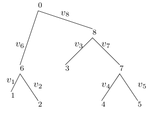
Exercises
21.2-1 Give an algorithm for the weighted small parsimony problem where we want to get minimum weight evolutionary labeling given a tree topology and a set of sequences associated to the leaves of the tree.
21.2-2 The gene content changes in species, a gene that can be found in a genome of a species might be abundant in another genome. In the simplest model an existing gene might be deleted from the genome and an abundant gene might appear. Give the small parsimony algorithm for this gene content evolution model.
21.2-3 Give an algorithm that obtains the Maximum Likelihood labelling on a tree.
21.2-4 Rewrite the small parsimony problem in the form of (21.40) replacing sums with minimalisation, and show that the Sankoff algorithm is based on the same rearrangement as the Felsenstein algorithm.
21.2-5 The Fitch algorithm [109] works in the following way: Each  node is associated with a set of characters,
  . The leaves are associated with a set containing the character associated to the leaves, and each internal character
  has the set:
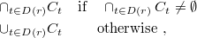
After reaching the root, we select an arbitrary character from  , where
  is the root of the tree, and we choose the same character that we chose at the parent node if the set of the child node has this character, otherwise an arbitrary character from the set of the child node. Show that we get a most parsimonious labelling. What is the running time of this algorithm?
21.2-6 Show that the Sankoff algorithm gives all possible most parsimonious labelling, while there are most parsimonious labellings that cannot be obtained with the Fitch algorithm.
Below we give algorithms on stochastic transformational grammars. Stochastic transformational grammars play a central role in modern bioinformatics. Two types of transformational grammars are widespread, the Hidden Markov Models (HMMs) are used for protein structure prediction and gene finding, while Stochastic Context Free Grammars (SCFGs) are used for RNA secondary structure prediction.
We give the formal definition of Hidden Markov Models (HMM): Let  denote a finite set of states. There are two distinguished states among the states, the start and the end states. The states are divided into two parts, emitting and non-emitting states. We assume that only the start and the end states are non-emitting, we will show that this assumption is not too strict.
The M transformation matrix contains the transition probabilities,  , that the Markov process will jump to state
  from state
  . Emitting states emit characters form a finite alphabet,
  . The probability that the state
  emits a character
  will be denoted by
  . The Markov process starts in the start state and ends in the end state, and walks according to the transition probabilities in M. Each emitting state emits a character, the emitted characters form a sequence. The process is hidden since the observer observes only the sequence and does not observe the path that the Markov process walked on. There are three important questions for HMMs that can be answered using dynamic programming algorithms.
The first question is the following: given an HMM and a sequence, what is the most likely path that emits the given sequence? The Viterbi algorithm gives the answer for this question. Recall that  is the
  -long prefix of sequence
  , and
, and  is the character in the
  th position. The dynamic programming answering the first question is based on that we can calculate the
  probability, the probability of the most probable path emitting prefix
  and being in state
  if we already calculated
  for all possible
  , since

The reason behind the above equation is that the probability of any path is the product of transition and emission probabilities. Among the products having the same last two terms (in our case  ) the maximal is the one for which the product of the other terms is maximal.
The initialisation of the dynamic programming is

Since the end state does not emit a character, the termination of the dynamic programming algorithm is

where  is the probability of the most likely path emitting the given sequence. One of the most likely paths can be obtained with a trace-back.
The second question is the following: given an HMM and a sequence, what is the probability that the HMM emits the sequence? This probability is the sum of the probabilities of paths that emit the given sequence. Since the number of paths emitting a given sequence might grow exponentially with the length of the sequence, the naive algorithm that finds all the possible emitting paths and sum their probabilities would be too slow.
The dynamic programming algorithm that calculates quickly the probability in question is called the Forward algorithm. It is very similar to the Viterbi algorithm, just there is a sum instead of maximalisation in it:

Since the END state does not emit, the termination is

where  is the probability that the HMM emits sequence
  .
.
The most likely path obtained by the Viterbi algorithm has more and less reliable parts. Therefore we are interested in the probability

This is the third question that we answer with dynamic programming algorithm. The above mentioned probability is the sum of the probabilities of paths that emit  in state
  divided by the probability that the HMM emits sequence
  . Since the number of such paths might grow exponentially, the naive algorithm that finds all the possible paths and sum their probability is too slow.
To answer the question, first we calculate for each suffix  and state
  what is the probability that the HMM emits suffix
  given that state
  emits
emits  . This can be calculated with the Backward algorithm, which is similar to the Forward algorithm just starts the recursion with the end of the sequence:

Let  denote the probability

Then

and from this

which is the needed probability.
It can be shown that every context-free grammar can be rewritten into Chomsky normal form. Each rule of a grammar in Chomsky normal form has the form  or
or  , where the
  s are non-terminal symbols, and
  is a terminal symbol. In a stochastic grammar, each derivation rule has a probability, a non-negative number such that the probabilities of derivation rules for each non-terminal sum up to
  .
.
Given a SCFG and a sequence, we can ask the questions analogous to the three questions we asked for HMMs: what is the probability of the most likely derivation, what is the probability of the derivation of the sequence and what is the probability that a sub-string has been derivated starting with  non-terminal, given that the SCFG derivated the sequence. The first question can be answered with the CYK (Cocke-Younger-Kasami) algorithm which is the Viterbi-equivalent algorithm for SCFGs. The second question can be answered with the Inside algorithm, this is the Forward-equivalent for SCFGs. The third question can be answered with the combination of the Inside and Outside algorithms, as expected, the
 Outside algorithm is analogous to the Backward algorithm. Though the introduced algorithms are equivalent with the algorithms used for HMMs, their running time is significantly greater.
Let  denote the probability of the rule
  , and let
  denote the probability of the rule
  . The
. The Inside algorithm calculates  for all
  and
and  , this is the probability that non-terminal
  derives the substring from
  till
till  . The initial conditions are:

for all  and
and  . The main recursion is:

where  is the number of non-terminals. The dynamic programming table is an upper triangle matrix for each non-terminal, the filling-in of the table starts with the main diagonal, and is continued with the other diagonals. The derivation probability is
  , where
  is the length of the sequence, and
  is the starting non-terminal. The running time of the algorithm is
  , the memory requirement is
  .
.
The Outside algorithm calculates  for all
  and
and  , this is the part of the derivation probability of deriving sequence
  which is “outside” of the derivation of substring from
  till
till  , starting the derivation from
  . A more formal definition for
  is that this is the sum of derivation probabilities in whom the substring from
  till
till  is derived from
  , divided by
  . Here we define
  as
as  . The initial conditions are:


The main recursion is:
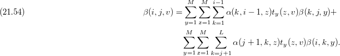
The reasoning for Eqn. 21.54 is the following. The  non-terminal was derivated from a
  non-terminal together with a
  non-terminal, and their derivation order could be both
  and
and  . The outside probability of non-terminal
  is product of the outside probability of
  , the derivation probability and the inside probability of
  . As we can see, inside probabilities are needed to calculate outside probabilities, this is a significant difference from the Backward algorithm that can be used without a Forward algorithm.
The CYK algorithm is very similar to the Inside algorithm, just there are maximalisations instead of summations:

The probability of the most likely derivation is  . The most likely derivation can be obtained with a trace-back.
Finally, the probability that the substring from  till
till  has been derived by
  given that the SCFG derived the sequence is:

Exercises
21.3-1 In a regular grammar, each derivation rule is either in a form  or in a form
  . Show that each HMM can be rewritten as a stochastic regular grammar. On the other hand, there are stochastic regular grammars that cannot be described as HMMs.
21.3-2 Give a dynamic programming algorithm that calculate for a stochastic regular grammar and a sequence 
-
the most likely derivation,
-
the probability of derivation,
-
the probability that character
 is derived by non-terminal
  .
.
21.3-3 An HMM can contain silent states that do not emit any character. Show that any HMM containing silent states other than the start and end states can be rewritten to an HMM that does not contain silent states above the start and end states and emits sequences with the same probabilities.
21.3-4 Pair Hidden Markov models are Markov models in which states can emit characters not only to one but two sequences. Some states emit only into one of the sequences, some states emit into both sequences. The observer sees only the sequences and does not see which state emits which characters and which characters are co-emitted. Give the Viterbi, Forward and Backward algorithms for pair-HMMs.
21.3-5 The Viterbi algorithm does not use that probabilities are probabilities, namely, they are non-negative and sum up to one. Moreover, the Viterbi algorithm works if we replace multiplications to additions (say that we calculate the logarithm of the probabilities). Give a modified HMM, namely, in which “probabilities” not necessary sum up to one, and they might be negative, too, and the Viterbi algorithm with additions are equivalent with the Gotoh algorithm.
21.3-6 Secondary structures of RNA sequences are set of basepairings, in which for all basepairing positions  and
and  ,
,  implies that either
  or
or  . The possible basepairings are
  ,
,  ,
,  ,
,  ,
,  and
and  . Give a dynamic programming algorithm that finds the secondary structure containing the maximum number of basepairings for an RNA sequence. This problem was first solved by Nussionov et al. [256].
21.3-7 The derivation rules of the Knudsen-Hein grammar are [202], [201]

where  has to be substituted with the possible characters of RNA sequences, and the
  s in the
  expression have to be replaced by possible basepairings. Show that the probability of the derivation of a sequence as well as the most likely derivation can be obtained without rewriting the grammar into Chomsky normal form.
In this section, we give dynamic programming algorithms for comparing structures. As we can see, aligning labelled rooted trees is a generalisation of sequence alignment. The recursions in the dynamic programming algorithm for comparing HMMs yields a linear equation system due to circular dependencies. However, we still can call it dynamic programming algorithm.
Let  be a finite alphabet, and
  ,
,  . Labelling of tree
  is a function that assigns a character of
  to each node
  . If we delete a node from the tree, then the children of the node will become children of the parental node. If we delete the root of the tree, then the tree becomes a forest. Let
  be a rooted tree labelled with characters from
  , and let
  represent the labelling.
  is an alignment of trees
  and
and  labelled with characters from
  if restricting the labeling of
  to the first (respectively, second) coordinates and deleting nodes labelled with '
  ' yields tree
  (respectively,
  ). Let
  be a similarity function. An optimal alignment of trees
  and
and  is the tree
  labelled with
  for which

is maximal. This tree is denoted by  . Note that a sequence can be represented with a unary tree, which has a single leaf. Therefore aligning trees is a generalisation of aligning sequences (with linear gap penalty).
Below we will concern only with trees in which each node has a degree at most  . The recursion in the dynamic programming algorithm goes on rooted subtrees. A rooted subtree of a tree contains a node
  of the tree and all nodes that are smaller than
  . The tree obtained by root
  is denoted by
  .
.
A tree to an empty tree can be aligned only in one way. Two leafes labelled by  and
and  can be aligned in three different way. The alignment might contain only one node labelled with
  or might contain two nodes, one of them is labelled with
  , the other with
  . One of the points is the root, the other the leaf.
Similarly, when we align a single leaf to a tree, then in the alignment  either the single character of the node is labelled together with a character of the tree or labelled together with '
  ' in an independent node. This node can be placed in several ways on tree
  , however the score of any of them is the same.
After this initialisation, the dynamic programming algorithm aligns greater rooted subtrees using the alignments of smaller rooted subtrees. We assume that we already know the score of the optimal alignments  ,
,  ,
,  ,
,  ,
,  ,
,  ,
,  and
and  when aligning subtrees
  and
and  , where
  and
and  are the children of
  and
and  and
and  are the children of
  . Should one of the nodes have only one child, the dynamic programming reduces the problem of aligning
  and
and  to less subproblems. We assume that the algorithm also knows the score of the optimal alignments of
  to the empty tree and the score of the optimal alignment of
  to the empty tree. Let the labelling of
  be
be  and the labelling of
  be
be  . We have to consider constant many subproblems for obtaining the score of the optimal alignment of
  and
and  . If one of the tree is aligned to one of the children's subtree of the other tree, then the other child and the root of the other tree is labelled together with '
  '. If character of
  is co-labelled with the character of
  , then the children nodes are aligned together, as well. The last situation is the case when the roots are not aligned in
  but one of the roots is the root of
  and the other root is its only child. The children might or might not be aligned together, this is five possible cases altogether.
Since the number of rooted subtrees equals to the number of nodes of the tree, the optimal alignment can be obtained in  time, where
  and
and  are the number of nodes in
  and
and  .
.
Let  and
and  be Hidden Markov Models. The co-emission probability of the two models is

where the summation is over all possible sequences and  is the probability that model
  emitted sequence
  . The probability that path
  emitted sequence
  is denoted by
  , a path from the START state till the
  state is denoted by
  . Since state
  can be reached on several paths, this definition is not well-defined, however, this will not cause a problem later on. Since the coemission probability is the sum of the product of emission of paths,
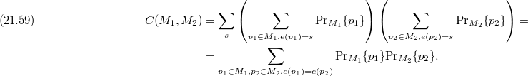
Let  denote the path that can be obtained with removing the last state from
  , and let
  be the state before
  in path
  . (We define similarly
  and
and  .) Hence
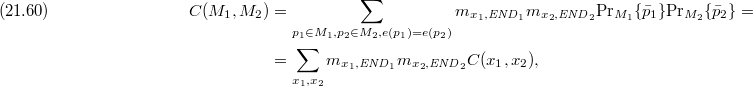
where  is the probability of jumping to END from
  , and
, and

 can be also obtained with this equation:

where  is the probability that
  emitted
  . Equation 21.62 defines a linear equation system for all pairs of emitting states
  and
and  . The initial conditions are:


Unlike the case of traditional dynamic programming, we do not fill in a dynamic programming table, but solve a linear equation system defined by Equation 21.62. Hence, the coemission probability can be calculated in  time, where
  and
and  are the number of emitting states of the models.
Exercises
21.4-1 Give a dynamic programming algorithm for the local similarities of two trees. This is the score of the most similar subtrees of the two trees. Here subtrees are any consecutive parts of the tree.
21.4-2 Ordered trees are rooted trees in which the children of a node are ordered. The ordered alignment of two ordered trees preserve the orderings in the aligned trees. Give an algorithm that obtains the optimal ordered alignment of two ordered trees and has running time being polynomial with both the maximum number of children and number of nodes.
21.4-3 Consider the infinite Euclidean space whose coordinates are the possible sequences. Each Hidden Markov model is a vector in this space the coordinates of the vector are the emission probabilities of the corresponding sequences. Obtain the angle between two HMMs in this space.
21.4-4 Give an algorithm that calculates the generating function of the length of the emitted sequences of an HMM, that is

where  is the probability that the Markov model emitted a sequence with length
  .
.
21.4-5 Give an algorithm that calculates the generating function of the length of the emitted sequences of a pair-HMM, that is
where  is the probability that the first emitted sequence has length
  , and the second emitted sequence has length
  .
.
In this section, we shell introduce algorithms whose input is a set of objects and distances between objects. The distances might be obtained from pairwise alignments of sequences, however, the introduced algorithms work for any kind of distances. The leaves of the tree are the given objects, and the topology and the lengths of the edges are obtained from the distances. Every weighted tree defines a metric on the leaves of the tree, we define the distance between two leaves as the sum of the weights of edges on the path connecting them. The goodness of algorithms can be measured as the deviation between the input distances and the distances obtained on the tree.
We define two special metrics, the ultrametric and additive metric. The clustering algorithms generate a tree that is always ultrametric. We shell prove that clustering algorithms gives back the ultrametric if the input distances follow a ultrametric, namely, the tree obtained by a clustering algorithm defines exactly the input distances.
Similarly, the Neighbour Joining algorithm creates a tree that represents an additive metric, and whenever the input distances follow an additive metric, the generated tree gives back the input distances.
For both proves, we need the following lemma:
Lemma 21.3 For any metric, there is at most one tree that represents it and has positive weights.
Proof. The proof is based on induction, the induction starts with three points. For three points, there is exactly one possible topology, a star-tree. Let the lengths of the edges connecting points  ,
,  and
and  with the internal node of the star three be
  ,
,  and
and  , respectively. The lengths of the edges defined by the


equation system, which has a unique solution since the determinant
is not  .
.
For  number of points, let us assume that there are two trees representing the same metric. We find a cherry motif on the first tree, with cherries
  and
and  . A cherry motif is a motif with two leafes whose connecting path has exactly one internal node. Every tree contains at least two cherry motives, a path on the tree that has the maximal number of internal nodes has cherry motives at both ends.
If there is only one internal node on the path connecting  and
and  on the other tree, then the length of the corresponding edges in the two cherry motives must be the same, since for any additional point
  , we must get the same subtree. We define a new metric by deleting points
  and
and  , and adding a new point
  . The distance between
  and any point
  is
is  , where
  is the length of the edge connecting
  with the internal point in the cherry motif. If we delete nodes
  and
and  , we get a tree that represent this metric and they are the same, according to the induction.
If the path between  and
and  contains more than one internal node on the other tree, then we find a contradiction. There is a
  point on the second tree for which
  . Consider a
  such that the path connecting
  and
and  contains node
  . From the first tree

while on the second tree

which contradicts that  .
.
Definition 21.4 A metric is ultrametric if for any three points,  ,
,  and
and 

It is easy to prove that the three distances between any three points are all equal or two of them equal and the third is smaller in any ultrametric.
Theorem 21.5 If the metric on a finite set of points is ultrametric, then there is exactly one tree that represents it. Furthermore, this tree can be rooted such that the distance between a point and the root is the same for all points.
Proof. Based on the Lemma 21.3, it is enough to construct one ultrametric tree for any ultrametric. We represent ultrametric trees as dendrograms. in this representation, the horizontal edges has length zero. For an example dendrogram, see Figure 21.2.
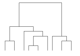
The proof is based on the induction on the number of leaves. Obviously, we can construct a dendrogram for two leaves. After constructing the dendrogram for  leaves, we add leaf
  to the dendrogram in the following way. We find a leaf
  in the dendrogram, for which
  is minimal. Then we walk up on the dendrogram till we reach the
  distance (we might go upper than the root). The node
  is connected to the dendrogram at this point, see Figure 21.3.
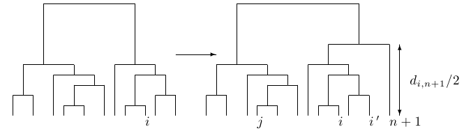
This dendrogram represents properly the distances between leaf  and any other leaf. Indeed, if leaf
  that is below the new internal node that bonnets leaf
  , then
  and from the ultrametric property and the minimality of
  it follows that
  . On the other hand, if leaf
  is not below the new internal point joining leaf
  , then
  , and from the ultrametric property it comes that
  .
.
It is easy to see that the construction in the proof needs  running time, where
  is the number of objects. We shell give another algorithm that finds the pair of objects
  and
and  for which
  is minimal. From the ultrametric property, for any
  ,
,  , hence we can replace the pair of objects
  and
and  to a new object, and the distance between this new object and any other object
  is well defined, it is
  . The objects
  and
and  are connected at height
  , and we treat this sub-dendrogram as a single object. We continue the iteration till we have a single object. This algorithm is slower than the previous algorithm, however, this is the basis of the clustering algorithms. The clustering algorithms create a dendrogram even if the input distances do not follow a ultrametric. On the other hand, if the input distances follow a ultrametric, then most of the clustering algorithms gives back this ultrametric.
As we mentioned, the clustering algorithms find the object pair  and
and  for which
  is minimal. The differences come from how the algorithms define the distance between the new object replacing the pair of objects
  and
and  and any other object. If the new object is denoted by
  , then the introduced clustering methods define
  in the following way:
-
Single link: .
. -
Complete link: .
. -
UPGMA:the new distance is the arithmetic mean of the distances between the elements in and
and  :
:  , where
  and
and  are the number of elements in
  and
and  .
. -
Single average: .
. -
Centroid:This method is used when the objects can be embedded into a Euclidean space. Then the distance between two objects can be defined as the distance between the centroids of the elements of the objects. It is not necessary to use the coordinates of the Euclidean space since the distance in question is the distance between point
  and the point intersecting the
  edge in
  proportion in the triangle obtained by points
  ,
,  és
és  (see Figure 21.4). This length can be calculated using only
  ,
,  and
and  . Hence the algorithm can be used even if the objects cannot be embedded into a Euclidean space.
 -
Median:The centroid of is the centroid of the centroids of
  and
and  . This method is related to the centroid method as the single average is related to the UPGMA method. It is again not necessary to know the coordinates of the elements, hence this method can be applied to distances that cannot be embedded into a Euclidean space.
It is easy to show that the first four method gives the dendrogram of the input distances whenever the input distances follow a ultrametric since  in this case. However, the
 Centroid and Median methods do not give the corresponding dendrogram for ultrametric input distances, since  will be smaller than
  (which equals to
  ).
).
The central problem of the clustering algorithms is that they give a dendrogram that might not be biologically correct. Indeed, the evolutionary tree of biological sequences can be a dendrogram only if the molecular clock hypothesis holds. The molecular clock hypothesis says that the sequences evolve with the same tempo at each branches of the tree, namely they collect the same number of mutations at a given time span. However, this is usually not true. Therefore biologists want an algorithm that give a ultrametric tree only if the input distances follow a ultrametric. The most popular such method is the Neighbour-Joining algorithm.
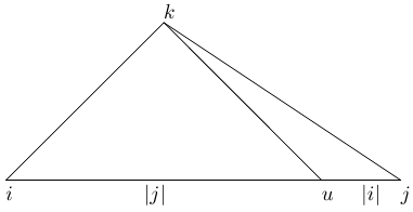
Definition 21.6 A metric is called additive or four-point metric, if for any four points  ,
,  ,
,  and
and 

Theorem 21.7 If a metric is additive on a finite set of objects, then there is exactly one tree that represents it.
Proof. Due to Lemma 21.3, there is at most one such tree, therefore it is enough to construct it. First we give the construction then we prove its goodness.
For three objects we can construct a tree according to (21.66)–(21.68). Assume that we constructed the tree for  objects, and we want to add leaf
  to the tree. First we find the topology and then we give the length of the new edge. For obtaining the new topology we start with any leaf
  , and let denote
  the neighbour of leaf
  . There are at least two other edges going out from
  , we find two leaves on the paths starting with these two outgoing edges, let
  and
and  denote these leaves, see Figure 21.5.
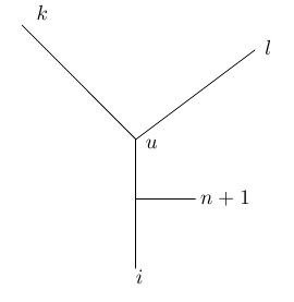
The leaf is connected to the edges between  and
and  if
if

Using similar inequalities, we can decide if leaf  is before
  looking from
  or looking from
  . If the degree of
  is greater than
  , then we find leaves
  on the other paths and we do the same investigations for
  ,
,  ,
,  and
and  points. From the additive property, it follows that inequality can hold at most for one cases. If it holds for
  , then we connect leaf
  to the edge connecting
  and
and  . If the inequality holds for another case, then we derive the maximal subtree of the tree that contains
  as a leaf and also contains the leaf for which the inequality holds. We define
  as
as  , then renaming
  to
to  we continue the searching for the connection place of leaf
  . If we get equality for all outgoing edges of
  , then we connect leaf
  to
to  .
.
After finding the topology, we obtain the length of the new edge. Leaf  is connected to the edge between
  and
and  , let
, let  denote the new internal point, see Figure 21.6/b.
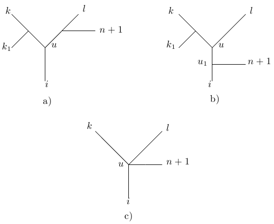
We define  as
as  . then the distances
  ,
,  , and
, and  can be calculated using (21.66)–(21.68). If the leaf
  is connected to
  , then
  .
.
Now we prove the correctness of the construction. First we show that  is well-defined, namely, for all node
  that is not in the new subtree containing leaves
  and
and  ,
,  . If the new subtree contains
  then for
  that was used to find the place of leaf
  will obviously hold (see Figure 21.6/a). Due to the additive metric property and the place of leaf

Using inequalities  és a
és a  , it follows that

Similarly for all leaves  that are not separated from
  by
by  , it holds that

It is due to the additive metric and the inequality

this later inequality comes from these inequalities


If the degree of  is greater than
  , then similar inequalities hold.
Due to the way of calculating the new edge lengths,  is represented properly on the new tree, hence
  is represented properly for all
  that is separated from leaf
  by
by  . Note that
  might be an earlier
  .
.
If leaf  is connected to the edge between
  and
and  (Figure 21.6/b), then due to the definition
  ,
,  is represented properly. From the equation

it follows that

hence  is represented properly. It can be similarly shown that for all points
  that are separated from
  by
by  , the
, the  is represented properly on the tree.
If leaf  is connected to node
  (Figure 21.6), then from the equations

it comes that both  and
and  are represents properly on the new tree, and with similar reasoning, it is easy to show that actually for all nodes
  that is separated from
  by
by  ,
,  is represented properly on the tree.
Hence we construct a tree containing leaf  from the tree containing the first
  leaves, thus proving Theorem 21.7.
It is easy to show that the above algorithm that constructs the tree representing an additive metric takes  running time. However, it works only if the input distances follow an additive metric, other wise inequality (21.74) might hold several times, hence we cannot decide where to join leaf
  to. We shell introduce an algorithm that has
  running time and gives back the additive tree whenever the input distances follow an additive metric, moreover it generates an additive tree that approximates the input distances if those are not follow an additive metric.
The Neighbour-Joining algorithm works in the following way: Given a set with  points and a distance function
  on the points. First we calculate the for each point
  the sum of the distances from the other points:

Then we find the pair of points for which

is minimal. The length of the edges from points  and
and  to the new point
  are
are

and

Then we recalculate distances. We drop points  and
and  , and add point
  . The distance between
  and any other point
  is defined as

Theorem 21.8 If  follows an additive metric, then the
 Neighbour-Joining algorithm generates a tree that gives back  .
.
Proof. From Theorem 21.7 there is exactly one tree that represents the distances. It is enough to prove that the Neighbour-Joining algorithm always pick a cherry motif on this tree, since a straightforward calculation shows that in this case the calculated edge lengths are proper.
First we prove if  and
and  follows a cherry motif then for all
  ,
,  és
és  . Indeed, rearranging
  , we have to prove that

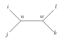
If  , then we get that

(see also Figure 21.7).  and the cases
  and
and  inside the sums cancel each other, hence we prove that the (21.89) inequality holds.
Now we prove the Theorem 21.8 in an indirect way. Suppose that  and
and  does not follow a cherry motif, however,
  is minimal. From the previous lemma, neither
  nor
nor  are in a cherry motif with other leaves. We find a cherry motif with leaves
  and
and  and internal node
  . Let
. Let  denote the last common node of paths going from
  to
to  and to
  . Since
  is minimal,

Rearranging this we get that

 and cases
  ,
,  ,
,  and
and  inside the sum cancel each other. For the other
  , the left hand side is

If  joins to the tree via the path connecting
  and
and  , then the expression 21.93 will be always negative, see also Figure 21.8. Let these cases be called I. class cases.
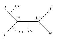
If  joins to the tree via the path between
  and
and  , then the expression 21.93 might be positive. Let these cases called II. class cases. To avoid contradiction, the sum of absolute values from I. class cases must be less than the sum from the II. class cases.
There is another  node on the path connecting
  and
and  , and we can find a cherry motif after node
  with leaves
  and
and  and internal node
  . Here again the II. class cases have to be more than the I. class cases, but this contradict to the situation with the first cherry motif. Hence
  and
and  form a cherry motif and we prove Theorem 21.8.
Exercises
21.5-1 Show that in a ultrametric, three distances coming from three points are all equal or two of them equal and the third is smaller. Prove the similar claim for the three sum of distances coming from four points in an additive metric.
21.5-2 Show that a ultrametric is always an additive metric.
21.5-3 Give an example for a metric that is not additive.
21.5-4 Is it true that all additive metric is a Euclidean metric?
21.5-5 Give the formula that calculates  from
from  ,
,  and
and  for the centroid method.
21.5-6 Give algorithms that decide in  whether or not a metric is
-
additive
-
ultrametric
( is the number of points.)
In this section, we cover topics that are usually not mentioned in bioinformatics books. We only mention the main results in a nutshell and do not prove theorems.
The genome of an organism consists of several genes. For each gene, only one strand of the double stranded DNA contains meaningful information, the other strand is the reverse complement. Since the DNA is chemically oriented, we can talk about the direction of a gene. If each gene has one copy in the genome then we can describe the order and directions of genes as a signed permutation, where the signs give the directions of genes.
Given two genomes with the same gene content, represented as a signed permutation then the problem is to give the minimal series of mutations that transform one genome into another. We consider three types of mutations:
-
Reversal A reversal acts on a consecutive part of the signed permutation. It reverse the order of genes on the given part as well as the signs of the genes.
-
Transposition A transposition swaps two consecutive block of genes.
-
Reverted transposition It swaps two consecutive blocks and one of the blocks is reverted. As for reversals, the signs in the reverted block also change.
If we assume that only mutations happened, then we can give an  running time algorithm that obtains a shortest series of mutations transforming one genome into another, where
  is the number of genes.
If we consider other types of mutations, then the complexity of problems is unknown. For transpositions, the best approximation is an  approximation [96], if we consider all possible types of mutations, then the best approximation is a
  -approximation [146]. For a wide range of and biologically meaningful weights, the weighted sorting problem for all types of mutations has a
  -approximation [26].
If we do not know the signs, then the problem is proved to be NP-complete [56]. Similarly, the optimal reversal median problem even for three genomes and signed permutations is NP-complete [55]. The optimal reversal median is a genome that minimises the sum of distances from a set of genomes.
Below we describe the Hannenhalli-Pevzner theorem for the reversal distance of two genomes. Instead of transforming permutation  into
into  , we transform
  into the identical permutation. Based on elementary group theory, it is easy to show that the two problems are equivalent. We assume that we already calculated
  , and we will denote it simply by
  .
.
We transform an  long signed permutation into a
  long unsigned permutation by replacing
  to
to  and
and  to
to  . Additionally, we frame the unsigned permutation into
  and
and  . The vertexes of the so-called graph of desire and reality are the numbers of the unsigned permutation together with
  and
and  . Starting with
  , we connect every other number in the graph, these are the reality edges. Starting also with
  , we connect
  with
with  with an arc, these are the desire edges. An example graph can be seen on Figure 21.9.
Figure 21.9. Representation of the signed permutation with an unsigned permutation, and its graph of desire and reality.
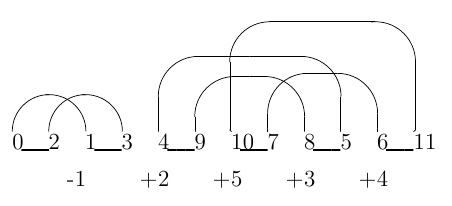
Since each vertex in the graph of desire and reality has a degree of two, the graph can be unequivocally decomposed into cycles. We call a cycle a directed cycle if on a walk on the cycle, we go at least once from left to right on a reality cycle and we go at least once from right to left on a reality cycle. Other cycles are unoriented cycles.
The span of a desire edge is the interval between its left and right vertexes. Two cycles overlap if there are two reality edges in the two cycles whose spans intersect. The vertexes of the overlap graph of a signed permutation are the cycles in its graph of desire and reality, two nodes are connected if the two cycles overlap. The overlap graph can be decomposed into components. A component is directed if it contains a directed cycle, otherwise it is unoriented. The span of a component is the interval between its leftmost and rightmost nodes in the graph of desire and reality. An unoriented component is a hurdle if its span does not contain any unoriented component or it contains all unoriented component. Other components are called protected non-hurdles.
A super-hurdle is hurdle for which it is true that if we delete this hurdle then one of the protected non-hurdles becomes a hurdle. A fortress is a permutation in which all hurdles are super-hurdles and their number is odd.
The Hannenhalli-Pevzner theorem is the following:
Theorem 21.9 Given a signed permutation  . The minimum number of mutations sorting this permutation into the identical permutation is

where  is the length of the permutation,
  is the number of cycles,
  is the number of hurdles, and
  if the permutation is a fortress, otherwise
  .
.
The proof of the theorem can be found in the book due to Pevzner.
The reversal distance was calculated in  time by Bader et al.. It is very easy to obtain
  in
in  time. The hard part is to calculate
  and
and  . The source of the problem is that the overlap graph might contain
  edges. Therefore the fast algorithm does not obtain the entire overlap graph, only a spanning tree on each component of it.
A genome of an organism usually contain significantly more than one million nucleic acids. Using a special biochemical technology, the order of nucleic acids can be obtained, however, the uncertainty grows with the length of the DNA, and becomes absolutely unreliable after about 500 nucleic acids.
A possible solution for overcoming this problem is the following: several copies are made from the original DNA sequence and they are fragmented into small parts that can be sequenced in the above described way. Then the original sequence must be reconstructed from its overlapping fragments. This technique is called shotgun sequencing.
The mathematical definition of the problem is that we want to find the shortest common super-sequence of a set of sequences. Sequence  is a super-sequence of
  if
if  is subsequence of
  . Recall that a subsequence is not necessarily a consecutive part of the sequence. Maier proved that the shortest common super-sequence problem is NP-complete is the size of the alphabet is at least
  and conjectured that it is the case if the size is at least
  . Later on it has been proved that the problem is NP-complete for all non-trivial alphabet [284].
Similar problem is the shortest common super-string problem, that is also an NP-complete problem [125]. This later has biological relevance, since we are looking for overlapping substrings. Several approximation algorithms have been published for the shortest common super-string problem. A greedy algorithm finds for each pair of strings the maximal possible overlap, then it tries to find a shortest common super-string by merging the overlapping strings in a greedy way [318]. The running time of the algorithm is  , where
  is the number of sequences and
  is the total length of the sequences. This greedy method is proved to be a
  -approximation [46]. A modified version being a
  -approximation also exist, and the conjecture is that the modified version is a
  -approximation [46].
The sequencing of DNA is not perfect, insertions, deletions and substitutions might happen during sequencing. Therefore Jiang and Li suggested the shortest  -approximative common super-string problem [182]. Kececioglu and Myers worked out a software package including several heuristic algorithm for the problem [196]. Later on Myers worked for Celera, which played a very important role in sequencing the human genome. A review paper on the topic can be found in [341].
Exercises
21.6-1 Show that a fortress contains at least three super-hurdle.
21.6-2 At least how long is a fortress?
PROBLEMS |
21-1 Concave Smith–Waterman
Give the Smith–Waterman-algorithm for concave gap penalty.
21-2 Concave Spouge
Give Spouge-algorithm for concave gap penalty.
21-3 Serving at a petrol station
There are two rows at a petrol station. Each car needs either petrol or diesel oil. At most two cars can be served at the same time, but only if they need different type of fuel, and the two cars are the first ones in the two rows or the first two in the same row. The serving time is the same not depending on whether two cars are being served or only one. Give a pair-HMM for which the Viterbi-algorithm provides a shortest serving scenario.
21-4 Moments of an HMM
Given an HMM and a sequence. Obtain the mean, variance,  th moment of the probabilities of paths emitting the given sequence.
21-5 Moments of a SCFG
Given a SCFG and a sequence. Obtain the mean, variance,  th moment of the probabilities of derivations of the given sequence.
21-6 Co-emission probability of two HMMs
Can this probability be calculated in  time where
  and
and  are the number of states in the HMMs?
21-7 Sorting reversals
A sorting reversal is a reversal that decreases the reversal distance of a signed permutation. How can a sorting reversal change the number of cycles and hurdles?
CHAPTER NOTES |
The first dynamic programming algorithm for aligning biological sequences was given by Needleman and Wunch in 1970 [252]. Though the concave gap penalty function is biologically more relevant, the affine gap penalty has been the standard soring scheme for aligning biological sequences. For example, one of the most popular multiple alignment program, CLUSTAL-W uses affine gap penalty and iterative sequence alignment [322]. The edit distance of two strings can calculated faster than  time, that is the famous “Four Russians' speedup” [19]. The running time of the algorithm is
  , however, it has such a big constant in the running time that it is not worth using it for sequence lengths appear in biological applications. The longest common subsequence problem can be solved using a dynamic programming algorithm similar to the dynamic programming algorithm for aligning sequences. Unlike that algorithm, the algorithm of Hunt and Szymanski creates a graph whose points are the characters of the sequences
  and
and  , and
, and  is connected to
  iff
iff  . Using this graph, the longest common subsequence can be find in
 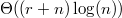 time, where
  is the number of edges in the graph and
  is the number of nodes [171]. Although the running time of this algorithm is
  , since the number of edges might be
  , in many cases the number of edges is only
  , and in this cases the running time is only
  . A very sophisticated version of the corner-cutting method is the diagonal extension technique, which fills in the dynamic programming table by diagonals and does not need a test value. An example for such an algorithm is the algorithm of Wu at al. [348]. The
 diff command in the Unix operating system is also based on diagonal extension [245], having a running time  , where
  and
and  are the lengths of the sequences and
  is the edit distance between the two sequences. The Knuth-Morris-Pratt string-searching algorithm searches a small pattern
  in a long string
  . Its running time is
  , where
  and
and  are the length of the sequences [203]. Landau and Vishkin modified this algorithm such that the modified version can find a pattern in
  that differs at most in
  position [216]. The running time of the algorithm is
  , the memory requirement is
  . Although dynamic programming algorithms are the most frequently used techniques for aligning sequences, it is also possible to attack the problem with integer linear programming. Kececioglu and his colleges gave the first linear programming algorithm for aligning sequences [195]. Their method has been extended to arbitrary gap penalty functions [9]. Lancia wrote a review paper on the topic [215] and Pachter and Sturmfels showed the relationship between the dynamic programming and integer linear programming approach in their book Algebraic Statistics for Computational Biology [263]. The structural alignment considers only the 3D structure of sequences. The optimal structural alignment problem is to find an alignment where we penalise gaps, however, the aligned characters scored not by their similarity but by how close their are in the superposed 3D structures. Several algorithms have been developed for the problem, one of them is the combinatorial extension (CE) algorithm [302]. For a given topology it is possible to find the Maximum Likelihood labeling [279]. This algorithm has been integrated into PAML, which is one of the most popular software package for phylogenetic analysis (http://abacus.gene.ucl.ac.uk/software/paml.html). The Maximum Likelihood tree problem is to find for a substitution model and a set of sequences the tree topology and edge lengths for which the likelihood is maximal. Surprisingly, it has only recently been proved that the problem is NP-complete [64], [288]. The similar problem, the Ancestral Maximum Likelihood problem has been showed to be NP-complete also only recently [4]. The AML problem is to find the tree topology, edge lengths and labellings for which the likelihood of a set of sequences is maximal in a given substitution model. The two most popular sequence alignment algorithms based on HMMs are the SAM [170] and the HMMER (http://hmmer.wustl.edu/) packages. An example for HMM for genome annotation is the work of Pedersen and Hein [269]. Comparative genome annotation can be done with pair-HMMs like the DoubleScan [242], (http://www.sanger.ac.uk/Software/analysis/doublescan/) and the Projector [243], (http://www.sanger.ac.uk/Software/analysis/projector/) programs. Goldman, Thorne and Jones were the first who published an HMM in which the emission probabilities are calculated from evolutionary informations [135]. It was used for protein secondary structure prediction. The HMM emits alignment columns, the emission probabilities can be calculated with the Felsenstein algorithm. The Knudsen-Hein grammar is used in the PFold program, which is for predicting RNA secondary structures [201]. This SCFG generates RNA multiple alignments, where the terminal symbols are alignment columns. The derivation probabilities can be calculated with the Felsenstein algorithm, the corresponding substitution model is a single nucleotide or a dinucleotide model, according to the derivation rules. The running time of the
 Forward algorithm grows squarely with the number of states in the HMM. However, this is not always the fastest algorithm. For a biologically important HMM, it is possible to reduce the  running time of the
 Forward algorithm to  with a more sophisticated algorithm [226], [227]. However, it is unknown whether or not similar acceleration exist for the
 Viterbi algorithm. The Zuker-Tinoco model [323] defines free energies for RNA secondary structure elements, and the free energy of an RNA structure is the sum of free energies of the elements. The Zuker-Sankoff algorithm calculates in  time the minimum free energy structure, using
  memory, where
  is the length of the RNA sequence. It is also possible to calculate the partition function of the Boltzmann distribution with the same running time and memory requirement [240]. For a special case of free energies, both the optimal structure and the partition function can be calculated in
  time, using still only
  memory [231]. Two base-pairings,
  and
and  forms a pseudo-knot if
  . Predicting the optimal RNA secondary structure in which arbitrary pseudo-knots are allowed is NP-complete [230]. For special types of pseudo-knots, polynomial running time algorithms exist [8], [230], [287], [329]. RNA secondary structures can be compared with aligning ordered forests [168]. Atteson gave a mathematical definition for the goodness of tree-constructing methods, and showed that the
 Neighbor-Joining algorithm is the best one for some definitions [22]. Elias and Lagergren recently published an improved algorithm for Neighbor-Joining that has only  running time [97]. There are three possible tree topologies for four species that are called quartets. If we know all the quartets of the tree, it is possible to reconstruct it. It is proved that it is enough to know only the short quartets of a tree that are the quartets of closely related species [98]. A genome might contain more than one DNA sequences, the DNA sequences are called chromosomes. A genome rearrangement might happen between chromosomes, too, such mutations are called translocations. Hannenhalli gave a
  running time algorithm for calculating the translocation and reversal distance [157]. Pisanti and Sagot generalised the problem and gave results for the translocation diameter [274]. The generalisation of sorting permutations is the problem of finding the minimum length generating word for an element of a group. The problem is known to be NP-complete [181]. Above the reversal distance and translocation distance problem, only for the block interchange distance exists a polynomial running time algorithm [65]. We mention that Bill Gates, the owner of Microsoft worked also on sorting permutations, actually, with prefix reversals [129].
Description of many algorithms of bioinformatics can be found in the book of Pevzner and Jones [272]. We wrote only about the most important topics of bioinformatics, and we did not cover several topics like recombination, pedigree analysis, character-based tree reconstructing methods, partial digesting, protein threading methods, DNA chip analysis, knowledge representation, biochemical pathways, scale-free networks, etc. We close the chapter with the words of Donald Knuth: “It is hard for me to say confidently that, after fifty more years of explosive growth of computer science, there will still be a lot of fascinating unsolved problems at peoples' fingertips, that it won't be pretty much working on refinements of well-explored things. Maybe all of the simple stuff and the really great stuff has been discovered. It may not be true, but I can't predict an unending growth. I can't be as confident about computer science as I can about biology. Biology easily has 500 years of exciting problems to work on, it's at that level.”
Table of Contents
Computer Graphics algorithms create and render virtual worlds stored in the computer memory. The virtual world model may contain shapes (points, line segments, surfaces, solid objects etc.), which are represented by digital numbers. Rendering computes the displayed image of the virtual world from a given virtual camera. The image consists of small rectangles, called pixels. A pixel has a unique colour, thus it is sufficient to solve the rendering problem for a single point in each pixel. This point is usually the centre of the pixel. Rendering finds that shape which is visible through this point and writes its visible colour into the pixel. In this chapter we discuss the creation of virtual worlds and the determination of the visible shapes.
The base set of our examination is the Euclidean space In computer algorithms the elements of this space should be described by numbers. The branch of geometry describing the elements of space by numbers is the analytic geometry. The basic concepts of analytic geometry are the vector and the coordinate system.
Definition 22.1 A vector is a translation that is defined by its direction and length. A vector is denoted by  .
.
The length of the vector is also called its absolute value, and is denoted by  . Vectors can be added, resulting in a new vector that corresponds to subsequent translations. Addition is denoted by
  . Vectors can be multiplied by scalar values, resulting also in a vector (
 ), which translates at the same direction as
  , but the length of translation is scaled by
  .
.
The dot product of two vectors is a scalar that is equal to the product of the lengths of the two vectors and the cosine of their angle:

Two vectors are said to be orthogonal if their dot product is zero.
On the other hand, the cross product of two vectors is a vector that is orthogonal to the plane of the two vectors and its length is equal to the product of the lengths of the two vectors and the sine of their angle:

There are two possible orthogonal vectors, from which that alternative is selected where our middle finger of the right hand would point if our thumb were pointing to the first and our forefinger to the second vector (right hand rule). Two vectors are said to be parallel if their cross product is zero.
Any vector  of a plane can be expressed as the linear combination of two, non-parallel vectors
  ,
,  in this plane, that is
Similarly, any vector  in the three-dimensional space can be unambiguously defined by the linear combination of three, not coplanar vectors:
Vectors  ,
,  ,
,  are called basis vectors, while scalars
  are referred to as coordinates. We shall assume that the basis vectors have unit length and they are orthogonal to each other. Having defined the basis vectors any other vector can unambiguously be expressed by three scalars, i.e. by its coordinates.
A point is specified by that vector which translates the reference point, called origin, to the given point. In this case the translating vector is the place vector of the given point.
The origin and the basis vectors constitute the Cartesian coordinate system, which is the basic tool to describe the points of the Euclidean plane or space by numbers.
The Cartesian coordinate system is the algebraic basis of the Euclidean geometry, which means that scalar triplets of Cartesian coordinates can be paired with the points of the space, and having made a correspondence between algebraic and geometric concepts, the theorems of the Euclidean geometry can be proven by algebraic means.
Exercises
22.1-1 Prove that there is a one-to-one mapping between Cartesian coordinate triplets and points of the three-dimensional space.
22.1-2 Prove that if the basis vectors have unit length and are orthogonal to each other, then  .
.
Coordinate systems provide means to specify points by numbers. Conditions on these numbers, on the other hand, may define sets of points. Conditions are formulated by equations. The coordinates found as the solution of these equations define the point set.
Let us now consider how these equations can be established.
A solid is a subset of the three-dimensional Euclidean space. To define this subset, continuous function  is used which maps the coordinates of points onto the set of real numbers. We say that a point belongs to the solid if the coordinates of the point satisfy the following implicit inequality:

Points satisfying inequality  are the internal points, while points defined by
  are the external points. Because of the continuity of function
  , points satisfying equality
  are between external and internal points and are called the boundary surface of the solid. Intuitively, function
  describes the signed distance between a point and the boundary surface.
We note that we usually do not consider any point set as a solid, but also require that the point set does not have lower dimensional degeneration (e.g. hanging lines or surfaces), i.e. that arbitrarily small neighborhoods of each point of the boundary surface contain internal points.
Figure 22.1 lists the defining functions of the sphere, the box, and the torus.
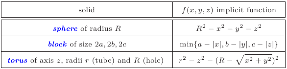
Points having coordinates that satisfy equation  are on the boundary surface. Surfaces can thus be defined by this implicit equation. Since points can also be given by the place vectors, the implicit equation can be formulated for the place vectors as well:

A surface may have many different equations. For example, equations  ,
,  , and M are algebraically different, but they have the same roots and thus define the same set of points.
A plane of normal vector  and place vector
  contains those points for which vector
  is perpendicular to the normal, thus their dot product is zero. Based on this, the points of a plane are defined by the following vector or scalar equations:

where  are the coordinates of the normal and
  . If the normal vector has unit length, then
  expresses the signed distance between the plane and the origin of the coordinate system. Two planes are said to be parallel if their normals are parallel.
In addition to using implicit equations, surfaces can also be defined by parametric forms. In this case, the Cartesian coordinates of surface points are functions of two independent variables. Denoting these free parameters by  and
and  , the parametric equations of the surface are:

The implicit equation of a surface can be obtained from the parametric equations by eliminating free parameters  . Figure 22.2 includes the parametric forms of the sphere, the cylinder and the cone.
![Parametric forms of the sphere, the cylinder, and the cone, where u,v\in[0,1] .](images/funcreps.png)
Parametric forms can also be defined directly for the place vectors:

Points of a triangle are the convex combinations of points  , and
, and  , that is

From this definition we can obtain the usual two-variate parametric form of a triangle substituting  by
by  ,
,  by
by  , and
, and  by
by  :
:

By intersecting two surfaces, we obtain a curve that may be defined formally by the implicit equations of the two intersecting surfaces

but this is needlessly complicated. Instead, let us consider the parametric forms of the two surfaces, given as  and
and  , respectively. The points of the intersection satisfy vector equation
  , which corresponds to three scalar equations, one for each coordinate of the three-dimensional space. Thus we can eliminate three from the four unknowns
  , and obtain a one-variate parametric equation for the coordinates of the curve points:

Similarly, we can use the vector form:

Figure 22.3 includes the parametric equations of the ellipse, the helix, and the line segment.
![Parametric forms of the ellipse, the helix, and the line segment, where t\in[0,1] .](images/funcrepg.png)
Note that we can define curves on a surface by fixing one of free parameters  . For example, by fixing
  the parametric form of the resulting curve is
  . These curves are called iso-parametric curves.
Two points define a line. Let us select one point and call the place vector of this point the place vector of the line. On the other hand, the vector between the two points is the direction vector. Any other point of the line can be obtained by a translation of the point of the place vector parallel to the direction vector. Denoting the place vector by  and the direction vector by
  , the equation of the line is:

Two lines are said to be parallel if their direction vectors are parallel.
Instead of the complete line, we can also specify the points of a line segment if parameter  is restricted to an interval. For example, the equation of the line segment between points
  and
and  is:
is:

According to this definition, the points of a line segment are the convex combinations of the endpoints.
In computer graphics we often need the normal vectors of the surfaces (i.e. the normal vector of the tangent plane of the surface). Let us take an example. A mirror reflects light in a way that the incident direction, the normal vector, and the reflection direction are in the same plane, and the angle between the normal and the incident direction equals to the angle between the normal and the reflection direction. To carry out such and similar computations, we need methods to obtain the normal of the surface.
The equation of the tangent plane is obtained as the first order Taylor approximation of the implicit equation around point  :
:


Points  and
and  are on the surface, thus
  and
and  , resulting in the following equation of the tangent plane:
Comparing this equation to equation (22.1), we can realize that the normal vector of the tangent plane is

The normal vector of parametric surfaces can be obtained by examining the iso-parametric curves. The tangent of curve  defined by fixing parameter
  is obtained by the first-order Taylor approximation:

Comparing this approximation to equation (22.2) describing a line, we conclude that the direction vector of the tangent line is  . The tangent lines of the curves running on a surface are in the tangent plane of the surface, making the normal vector perpendicular to the direction vectors of these lines. In order to find the normal vector, both the tangent line of curve
  and the tangent line of curve
  are computed, and their cross product is evaluated since the result of the cross product is perpendicular to the multiplied vectors. The normal of surface
  is then

Parametric and implicit equations trace back the geometric design of the virtual world to the establishment of these equations. However, these equations are often not intuitive enough, thus they cannot be used directly during design. It would not be reasonable to expect the designer working on a human face or on a car to directly specify the equations of these objects. Clearly, indirect methods are needed which require intuitive data from the designer and define these equations automatically. One category of these indirect approaches apply control points. Another category of methods work with elementary building blocks (box, sphere, cone, etc.) and with set operations.
Let us discuss first how the method based on control points can define curves. Suppose that the designer specified points  , and that parametric curve of equation
  should be found which “follows” these points. For the time being, the curve is not required to go through these control points.
We use the analogy of the centre of mass of mechanical systems to construct our curve. Assume that we have sand of unit mass, which is distributed at the control points. If a control point has most of the sand, then the centre of mass is close to this point. Controlling the distribution of the sand as a function of parameter  to give the main influence to different control points one after the other, the centre of mass will travel through a curve running close to the control points.
Let us put weights  at control points at parameter
  . These weighting functions are also called the basis functions of the curve. Since unit weight is distributed, we require that for each
  the following identity holds:

For some  , the respective point of the curve curve is the centre of mass of this mechanical system:
Note that the reason of distributing sand of unit mass is that this decision makes the denominator of the fraction equal to 1. To make the analogy complete, the basis functions cannot be negative since the mass is always non-negative. The centre of mass of a point system is always in the convex hull of the participating points, thus if the basis functions are non-negative, then the curve remains in the convex hull of the control points.
Footnote. The convex hull of a point system is by definition the minimal convex set containing the point system.
The properties of the curves are determined by the basis functions. Let us now discuss two popular basis function systems, namely the basis functions of the Bézier-curves and the B-spline curves.
Pierre Bézier, a designer working at Renault, proposed the Bernstein polynomials as basis functions. Bernstein polynomials can be obtained as the expansion of  according to binomial theorem:
The basis functions of Bézier curves are the terms of this sum ( ):
):

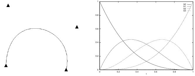
According to the introduction of Bernstein polynomials, it is obvious that they really meet condition 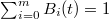 and
and  in
in  , which guarantees that Bézier curves are always in the convex hulls of their control points. The basis functions and the shape of the Bézier curve are shown in Figure 22.4. At parameter value
  the first basis function is 1, while the others are zero, therefore the curve starts at the first control point. Similarly, at parameter value
  the curve arrives at the last control point. At other parameter values, all basis functions are positive, thus they simultaneously affect the curve. Consequently, the curve usually does not go through the other control points.
The basis functions of the B-spline can be constructed applying a sequence of linear blending. A B-spline weights the  number of control points by
  -degree polynomials. Value
  is called the order of the curve. Let us take a non-decreasing series of
  parameter values, called the knot vector:

Figure 22.5. Construction of B-spline basis functions. A higher order basis function is obtained by blending two consecutive basis functions on the previous level using a linearly increasing and a linearly decreasing weighting, respectively. Here the number of control points is 5, i.e. . Arrows indicate useful interval where we can find number of basis functions that add up to 1. The right side of the figure depicts control points with triangles and curve points corresponding to the knot values by circles.
![Construction of B-spline basis functions. A higher order basis function is obtained by blending two consecutive basis functions on the previous level using a linearly increasing and a linearly decreasing weighting, respectively. Here the number of control points is 5, i.e. m=4 . Arrows indicate useful interval [t_{k-1},t_{m+1}] where we can find m+1 number of basis functions that add up to 1. The right side of the figure depicts control points with triangles and curve points corresponding to the knot values by circles.](images/an4Eng.png)
By definition, the  th first order basis function is 1 in the
  th interval, and zero elsewhere (Figure 22.5):
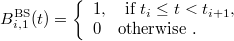
Using this definition,  number of first order basis functions are established, which are non-negative zero-degree polynomials that sum up to 1 for all
  parameters. These basis functions have too low degree since the centre of mass is not even a curve, but jumps from control point to control point.
The order of basis functions, as well as the smoothness of the curve, can be increased by blending two consecutive basis functions with linear weighting (Figure 22.5). The first basis function is weighted by linearly increasing factor 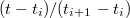 in domain
  , where the basis function is non-zero. The next basis function, on the other hand, is scaled by linearly decreasing factor
  in its domain
  where it is non zero. The two weighted basis functions are added to obtain the tent-like second order basis functions. Note that while a first order basis function is non-zero in a single interval, the second order basis functions expand to two intervals. Since the construction makes a new basis function from every pair of consecutive lower order basis functions, the number of new basis functions is one less than that of the original ones. We have just
  second order basis functions. Except for the first and the last first order basis functions, all of them are used once with linearly increasing and once with linearly decreasing weighting, thus with the exception of the first and the last intervals, i.e. in
  , the new basis functions also sum up to 1.
The second order basis functions are first degree polynomials. The degree of basis functions, i.e. the order of the curve, can be arbitrarily increased by the recursive application of the presented blending method. The dependence of the next order basis functions on the previous order ones is as follows:

Note that we always take two consecutive basis functions and weight them in their non-zero domain (i.e. in the interval where they are non-zero) with linearly increasing factor  and with linearly decreasing factor
  , respectively. The two weighted functions are summed to obtain the higher order, and therefore smoother basis function. Repeating this operation
  times,
  -order basis functions are generated, which sum up to 1 in interval
  . The knot vector may have elements that are the same, thus the length of the intervals may be zero. Such intervals result in 0/0 like fractions, which must be replaced by value 1 in the implementation of the construction.
The value of the  th
th  -order basis function at parameter
  can be computed with the following Cox-deBoor-Mansfield recursion:
B-Spline(
)
1IF
Trivial case. 2
THENIF3
THENRETURN1 4ELSERETURN0 5IF6
THEN
Previous with linearly increasing weight. 7
ELSE
Here: 0/0 = 1. 8
IF9
THEN
Next with linearly decreasing weight. 10
ELSE
Here: 0/0 = 1. 11
B-spline()B-spline()Recursion. 12
RETURN


Figure 22.6. A B-spline interpolation. Based on points to be interpolated, control points are computed to make the start and end points of the segments equal to the interpolated points.
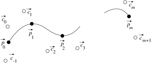
In practice, we usually use fourth-order basis functions  , which are third-degree polynomials, and define curves that can be continuously differentiated twice. The reason is that bent rods and motion paths following the Newton laws also have this property.
While the number of control points is greater than the order of the curve, the basis functions are non-zero only in a part of the valid parameter set. This means that a control point affects just a part of the curve. Moving this control point, the change of the curve is local. Local control is a very important property since the designer can adjust the shape of the curve without destroying its general form.
A fourth-order B-spline usually does not go through its control points. If we wish to use it for interpolation, the control points should be calculated from the points to be interpolated. Suppose that we need a curve which visits points  at parameter values
  , respectively (Figure 22.6). To find such a curve, control points
  should be found to meet the following interpolation criteria:
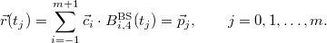
These criteria can be formalized as  linear equations with
  unknowns, thus the solution is ambiguous. To make the solution unambiguous, two additional conditions should be imposed. For example, we can set the derivatives (for motion paths, the speed) at the start and end points.
B-spline curves can be further generalized by defining the influence of the  th control point as the product of B-spline basis function
  and additional weight
  of the control point. The curve obtained this way is called the Non-Uniform Rational B-Spline, abbreviated as NURBS, which is very popular in commercial geometric modelling systems.
Using the mechanical analogy again, the mass put at the  th control point is
  , thus the centre of mass is:
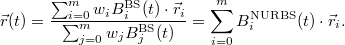
The correspondence between B-spline and NURBS basis functions is as follows:
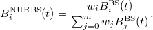
Since B-spline basis functions are piece-wise polynomial functions, NURBS basis functions are piece-wise rational functions. NURBS can describe quadratic curves (e.g. circle, ellipse, etc.) without any approximation error.
Parametric surfaces are defined by two variate functions  . Instead of specifying this function directly, we can take finite number of control points
  which are weighted with the basis functions to obtain the parametric function:

Similarly to curves, basis functions are expected to sum up to 1, i.e. 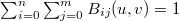 everywhere. If this requirement is met, we can imagine that the control points have masses
  depending on parameters
  , and the centre of mass is the surface point corresponding to parameter pair
  .
.
Basis functions  are similar to those of curves. Let us fix parameter
  . Changing parameter
  , curve
  is obtained on the surface. This curve can be defined by the discussed curve definition methods:

where  is the basis function of the selected curve type.
Of course, fixing  differently we obtain another curve of the surface. Since a curve of a given type is unambiguously defined by the control points, control points
  must depend on the fixed
  value. As parameter
  changes, control point
  also runs on a curve, which can be defined by control points
 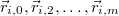 :
:
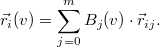
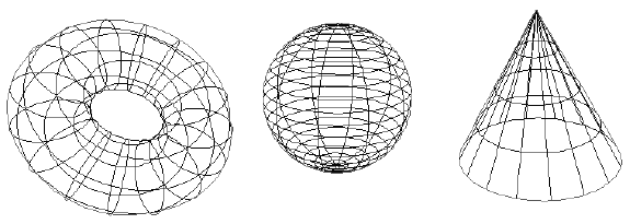
Substituting this into equation (22.8), the parametric equation of the surface is:
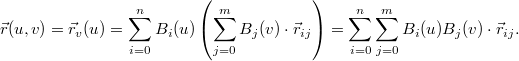
Unlike curves, the control points of a surface form a two-dimensional grid. The two-dimensional basis functions are obtained as the product of one-variate basis functions parameterized by  and
and  , respectively.
Free form solids – similarly to parametric curves and surfaces – can also be specified by finite number of control points. For each control point  , let us assign influence function
  , which expresses the influence of this control point at distance
  . By definition, the solid contains those points where the total influence of the control points is not smaller than threshold
  (Figure 22.8):
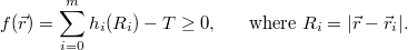
With a single control point a sphere can be modeled. Spheres of multiple control points are combined together to result in an object having smooth surface (Figure 22.8). The influence of a single point can be defined by an arbitrary decreasing function that converges to zero at infinity. For example, Blinn proposed the
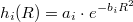
influence functions for his blob method.
Another type of solid modelling is constructive solid geometry (CSG for short), which builds complex solids from primitive solids applying set operations (e.g. union, intersection, difference, complement, etc.) (Figures 22.9 and 22.10). Primitives usually include the box, the sphere, the cone, the cylinder, the half-space, etc. whose functions are known.
Figure 22.8. The influence decreases with the distance. Spheres of influence of similar signs increase, of different signs decrease each other.
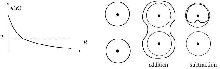
Figure 22.9. The operations of constructive solid geometry for a cone of implicit function and for a sphere of implicit function : union (), intersection (), and difference ().
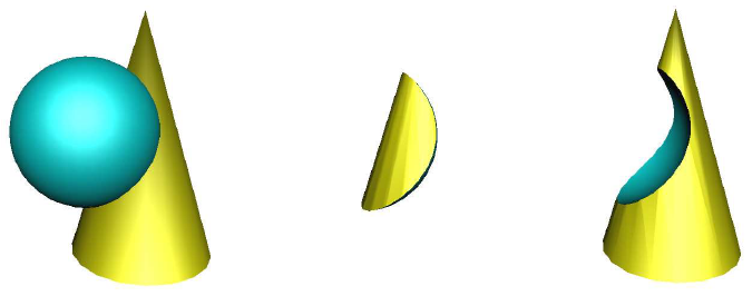
Figure 22.10. Constructing a complex solid by set operations. The root and the leaf of the CSG tree represents the complex solid, and the primitives, respectively. Other nodes define the set operations (U: union, : difference).
The results of the set operations can be obtained from the implicit functions of the solids taking part of this operation:
-
intersection of
 and
and  :
:  ;
; -
union of
 and
and  :
:  .
. -
complement of
 :
:  .
. -
difference of
 and
and  :
:  .
.
Implicit functions also allow to morph between two solids. Suppose that two objects, for example, a box of implicit function  and a sphere of implicit function
  need to be morphed. To define a new object, which is similar to the first object with percentage
  and to the second object with percentage
  , the two implicit equations are weighted appropriately:

Exercises
22.2-1 Find the parametric equation of a torus.
22.2-2 Prove that the fourth-order B-spline with knot-vector [0,0,0,0,1,1,1,1] is a Bézier curve.
22.2-3 Give the equations for the surface points and the normals of the waving flag and waving water disturbed in a single point.
22.2-4 Prove that the tangents of a Bézier curve at the start and the end are the lines connecting the first two and the last two control points, respectively.
22.2-5 Give the algebraic forms of the basis functions of the second, the third, and the fourth-order B-splines.
22.2-6 Develop an algorithm computing the path length of a Bézier curve and a B-spline. Based on the path length computation move a point along the curve with uniform speed.
In Section 22.2 we met free-form surface and curve definition methods. During image synthesis, however, line segments and polygons play important roles. In this section we present methods that bridge the gap between these two types of representations. These methods convert geometric models to lines and polygons, or further process line and polygon models. Line segments connected to each other in a way that the end point of a line segment is the start point of the next one are called polylines. Polygons connected at edges, on the other hand, are called meshes. Vectorization methods approximate free-form curves by polylines. A polyline is defined by its vertices. Tessellation algorithms, on the other hand, approximate free-form surfaces by meshes. For illumination computation, we often need the normal vector of the original surface, which is usually stored with the vertices. Consequently, a mesh contains a list of polygons, where each polygon is given by its vertices and the normal of the original surface at these vertices. Methods processing meshes use other topology information as well, for example, which polygons share an edge or a vertex.
Definition 22.2 A polygon is a bounded part of the plane, i.e. it does not contain a line, and is bordered by line segments. A polygon is defined by the vertices of the bordering polylines.
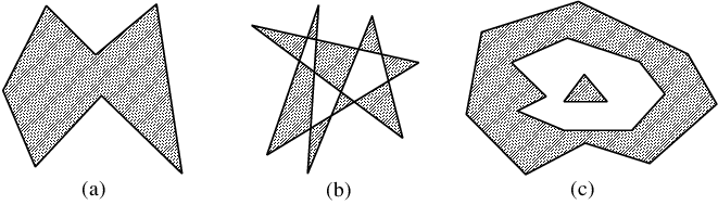
Definition 22.3 A polygon is single connected if its border is a single closed polyline (Figure 22.11).
Definition 22.4 A polygon is simple if it is single connected and the bordering polyline does not intersect itself (Figure 22.11(a)).
For a point of the plane, we can detect whether or not this point is inside the polygon by starting a half-line from this point and counting the number of intersections with the boundary. If the number of intersections is an odd number, then the point is inside, otherwise it is outside.
In the three-dimensional space we can form meshes, where different polygons are in different planes. In this case, two polygons are said to be neighboring if they share an edge.
Definition 22.5 A polyhedron is a bounded part of the space, which is bordered by polygons.
Similarly to polygons, a point can be tested for polyhedron inclusion by casting a half line from this point and counting the number of intersections with the face polygons. If the number of intersections is odd, then the point is inside the polyhedron, otherwise it is outside.
Parametric functions map interval  onto the points of the curve. During vectorization the parameter interval is discretized. The simplest discretization scheme generates
  evenly spaced parameter values
  (
(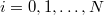 ), and defines the approximating polyline by the points obtained by substituting these parameter values into parametric equation
  .
.
Let us first consider the conversion of simple polygons to triangles. This is easy if the polygon is convex since we can select an arbitrary vertex and connect it with all other vertices, which decomposes the polygon to triangles in linear time. Unfortunately, this approach does not work for concave polygons since in this case the line segment connecting two vertices may go outside the polygon, thus cannot be the edge of one decomposing triangle.
Let us start the discussion of triangle conversion algorithms with two definitions:
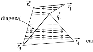
Definition 22.6 The diagonal of a polygon is a line segment connecting two vertices and is completely contained by the polygon (line segment  and
and  of Figure 22.12).
The diagonal property can be checked for a line segment connecting two vertices by trying to intersect the line segment with all edges and showing that intersection is possible only at the endpoints, and additionally showing that one internal point of the candidate is inside the polygon. For example, this test point can be the midpoint of the line segment.
Definition 22.7 A vertex of the polygon is an ear if the line segment between the previous and the next vertices is a diagonal (vertex  of Figure 22.12).
Clearly, only those vertices may be ears where the inner angle is not greater than 180 degrees. Such vertices are called convex vertices.
For simple polygons the following theorems hold:
Theorem 22.8 A simple polygon always has a diagonal.
Proof. Let the vertex standing at the left end (having the minimal  coordinate) be
  , and its two neighboring vertices be
  and
and  , respectively (Figure 22.13). Since
  is standing at the left end, it is surely a convex vertex. If
  is an ear, then line segment
  is a diagonal (left of Figure 22.13), thus the theorem is proven for this case. Since
  is a convex vertex, it is not an ear only if triangle
  ,
,  ,
,  contains at least one polygon vertex (right of Figure22.13). Let us select from the contained vertices that vertex
  which is the farthest from the line defined by points
  . Since there are no contained points which are farther from line
  than
than  , no edge can be between points
  and
and  , thus
  must be a diagonal.
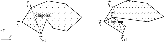
Theorem 22.9 A simple polygon can always be decomposed to triangles with its diagonals. If the number of vertices is  , then the number of triangles is
  .
.
Proof. This theorem is proven by induction. The theorem is obviously true when  , i.e. when the polygon is a triangle. Let us assume that the statement is also true for polygons having
  (
( ) number of vertices, and consider a polygon with
  vertices. According to Theorem 22.8, this polygon of
  vertices has a diagonal, thus we can subdivide this polygon into a polygon of
  vertices and a polygon of
  vertices, where
  , and
, and  since the vertices at the ends of the diagonal participate in both polygons. According to the assumption of the induction, these two polygons can be separately decomposed to triangles. Joining the two sets of triangles, we can obtain the triangle decomposition of the original polygon. The number of triangles is
  .
.
The discussed proof is constructive thus it inspires a subdivision algorithm: let us find a diagonal, subdivide the polygon along this diagonal, and continue the same operation for the two new polygons.
Unfortunately the running time of such an algorithm is in  since the number of diagonal candidates is
  , and the time needed by checking whether or not a line segment is a diagonal is in
  .
.
We also present a better algorithm, which decomposes a convex or concave polygon defined by vertices  . This algorithm is called ear cutting. The algorithm looks for ear triangles and cuts them until the polygon gets simplified to a single triangle. The algorithm starts at vertex
  . When a vertex is processed, it is first checked whether or not the previous vertex is an ear. If it is not an ear, then the next vertex is chosen. If the previous vertex is an ear, then the current vertex together with the two previous ones form a triangle that can be cut, and the previous vertex is deleted. If after deletion the new previous vertex has index 0, then the next vertex is selected as the current vertex.
The presented algorithm keeps cutting triangles until no more ears are left. The termination of the algorithm is guaranteed by the following two ears theorem:
Theorem 22.10 A simple polygon having at least four vertices always has at least two not neighboring ears that can be cut independently.
Proof. The proof presented here has been given by Joseph O'Rourke. According to theorem 22.9, every simple polygon can be subdivided to triangles such that the edges of these triangles are either the edges or the diagonals of the polygon. Let us make a correspondence between the triangles and the nodes of a graph where two nodes are connected if and only if the two triangles corresponding to these nodes share an edge. The resulting graph is connected and cannot contain circles. Graphs of these properties are trees. The name of this tree graph is the dual tree. Since the polygon has at least four vertices, the number of nodes in this tree is at least two. Any tree containing at least two nodes has at least two leaves. Leaves of this tree, on the other hand, correspond to triangles having an ear vertex.
Footnote. A leaf is a node connected by exactly one edge.
According to the two ears theorem, the presented algorithm finds an ear in  steps. Cutting an ear the number of vertices is reduced by one, thus the algorithm terminates in
  steps.
Parametric forms of surfaces map parameter rectangle  onto the points of the surface.
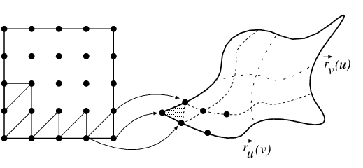
In order to tessellate the surface, first the parameter rectangle is subdivided to triangles. Then applying the parametric equations for the vertices of the parameter triangles, the approximating triangle mesh can be obtained. The simplest subdivision of the parametric rectangle decomposes the domain of parameter  to
to  parts, and the domain of parameter
  to
to  intervals, resulting in the following parameter pairs:

Taking these parameter pairs and substituting them into the parametric equations, point triplets  ,
,  ,
,  , and point triplets
  ,
,  ,
,  are used to define triangles.
The tessellation process can be made adaptive as well, which uses small triangles only where the high curvature of the surface justifies them. Let us start with the parameter rectangle and subdivide it to two triangles. In order to check the accuracy of the resulting triangle mesh, surface points corresponding to the edge midpoints of the parameter triangles are compared to the edge midpoints of the approximating triangles. Formally the following distance is computed (Figure 22.15):
where  and
and  are the parameters of the two endpoints of the edge.
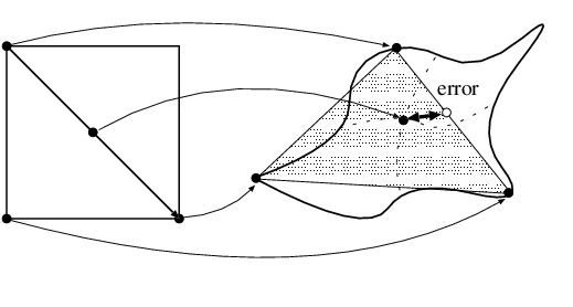
A large distance value indicates that the triangle mesh poorly approximates the parametric surface, thus triangles must be subdivided further. This subdivision can be executed by cutting the triangle to two triangles by a line connecting the midpoint of the edge of the largest error and the opposing vertex. Alternatively, a triangle can be subdivided to four triangles with its halving lines. The adaptive tessellation is not necessarily robust since it can happen that the distance at the midpoint is small, but at other points is still quite large.
When the adaptive tessellation is executed, it may happen that one triangle is subdivided while its neighbour is not, which results in holes. Such problematic midpoints are called T vertices (Figure 22.16).
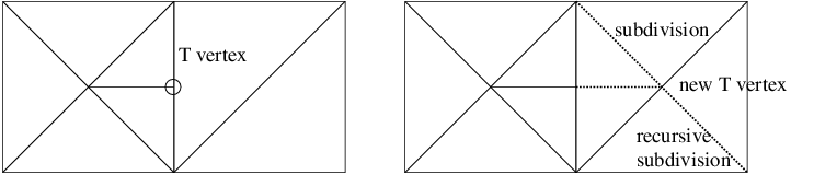
If the subdivision criterion is based only on edge properties, then T vertices cannot show up. However, if other properties are also taken into account, then T vertices may appear. In such cases, T vertices can be eliminated by recursively forcing the subdivision also for those neighbouring triangles that share subdivided edges.
This section presents algorithms that smooth polyline and mesh models.
Figure 22.17. Construction of a subdivision curve: at each step midpoints are obtained, then the original vertices are moved to the weighted average of neighbouring midpoints and of the original vertex.
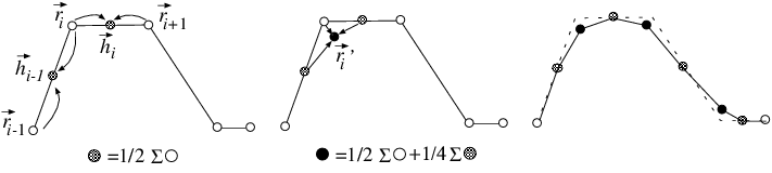
Let us consider a polyline of vertices  . A smoother polyline is generated by the following vertex doubling approach (Figure 22.17). Every line segment of the polyline is halved, and midpoints
  are added to the polyline as new vertices. Then the old vertices are moved taking into account their old position and the positions of the two enclosing midpoints, applying the following weighting:

The new polyline looks much smoother. If we should not be satisfied with the smoothness yet, the same procedure can be repeated recursively. As can be shown, the result of the recursive process converges to the B-spline curve.
Figure 22.18. One smoothing step of the Catmull-Clark subdivision. First the face points are obtained, then the edge midpoints are moved, and finally the original vertices are refined according to the weighted sum of its neighbouring edge and face points.
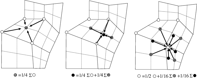
The polyline subdivision approach can also be extended for smoothing three-dimensional meshes. This method is called Catmull-Clark subdivision algorithm. Let us consider a three-dimensional quadrilateral mesh (Figure 22.18). In the first step the midpoints of the edges are obtained, which are called edge points. Then face points are generated as the average of the vertices of each face polygon. Connecting the edge points with the face points, we still have the original surface, but now defined by four times more quadrilaterals. The smoothing step modifies first the edge points setting them to the average of the vertices at the ends of the edge and of the face points of those quads that share this edge. Then the original vertices are moved to the weighted average of the face points of those faces that share this vertex, and of edge points of those edges that are connected to this vertex. The weight of the original vertex is 1/2, the weights of edge and face points are 1/16. Again, this operation may be repeated until the surface looks smooth enough (Figure 22.19).
Figure 22.19. Original mesh and its subdivision applying the smoothing step once, twice and three times, respectively.
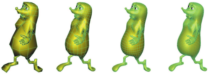
If we do not want to smooth the mesh at an edge or around a vertex, then the averaging operation ignores the vertices on the other side of the edge to be preserved.
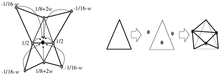
The Catmull-Clark subdivision surface usually does not interpolate the original vertices. This drawback is eliminated by the butterfly subdivision, which works on triangle meshes. First the butterfly algorithm puts new edge points close to the midpoints of the original edges, then the original triangle is replaced by four triangles defined by the original vertices and the new edge points (Figure 22.20). The position of the new edge points depend on the vertices of those two triangles incident to this edge, and on those four triangles which share edges with these two. The arrangement of the triangles affecting the edge point resembles a butterfly, hence the name of this algorithm. The edge point coordinates are obtained as a weighted sum of the edge endpoints multiplied by  , the third vertices of the triangles sharing this edge using weight
  , and finally of the other vertices of the additional triangles with weight
  . Parameter
  can control the curvature of the resulting mesh. Setting
  , the mesh keeps its original faceted look, while
  results in strong rounding.
A surface defined by implicit equation  can be converted to a triangle mesh by finding points on the surface densely, i.e. generating points satisfying
  , then assuming the close points to be vertices of the triangles.
First function  is evaluated at the grid points of the Cartesian coordinate system and the results are stored in a three-dimensional array, called voxel array. Let us call two grid points as neighbours if two of their coordinates are identical and the difference in their third coordinate is 1. The function is evaluated at the grid points and is assumed to be linear between them. The normal vectors needed for shading are obtained as the gradient of function
  (equation 22.4), which are also interpolated between the grid points.
When we work with the voxel array, original function  is replaced by its tri-linear approximation (tri-linear means that fixing any two coordinates the function is linear with respect to the third coordinate). Due to the linear approximation an edge connecting two neighbouring grid points can intersect the surface at most once since linear equations may have at most one root. The density of the grid points should reflect this observation, then we have to define them so densely not to miss roots, that is, not to change the topology of the surface.
Figure 22.21. Possible intersections of the per-voxel tri-linear implicit surface and the voxel edges. From the possible 256 cases, these 15 topologically different cases can be identified, from which the others can be obtained by rotations. Grid points where the implicit function has the same sign are depicted by circles.
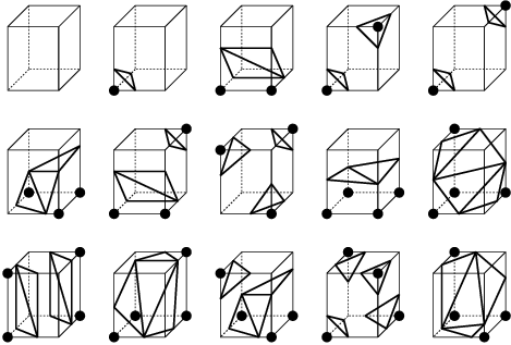
The method approximating the surface by a triangle mesh is called marching cubes algorithm. This algorithm first decides whether a grid point is inside or outside of the solid by checking the sign of function  . If two neighbouring grid points are of different type, the surface must go between them. The intersection of the surface and the edge between the neighbouring points, as well as the normal vector at the intersection are determined by linear interpolation. If one grid point is at
  , the other is at
  , and function
  has different signs at these points, then the intersection of the tri-linear surface and line segment
  is:
is:
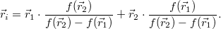
The normal vector here is:

Having found the intersection points, triangles are defined using these points as vertices. When defining these triangles, we have to take into account that a tri-linear surface may intersect the voxel edges at most once. Such intersection occurs if function  has different signs at the two grid points. The number of possible variations of positive/negative signs at the 8 vertices of a cube is 256, from which 15 topologically different cases can be identified (Figure 22.21).
The algorithm inspects grid points one by one and assigns the sign of the function to them encoding negative sign by 0 and non-negative sign by 1. The resulting 8 bit code is a number in 0–255 which identifies the current case of intersection. If the code is 0, all voxel vertices are outside the solid, thus no voxel surface intersection is possible. Similarly, if the code is 255, the solid is completely inside, making the intersections impossible. To handle other codes, a table can be built which describes where the intersections show up and how they form triangles.
Exercises
22.3-1 Prove the two ears theorem by induction.
22.3-2 Develop an adaptive curve tessellation algorithm.
22.3-3 Prove that the Catmull-Clark subdivision curve and surface converge to a B-spline curve and surface, respectively.
22.3-4 Build a table to control the marching cubes algorithm, which describes where the intersections show up and how they form triangles.
22.3-5 Propose a marching cubes algorithm that does not require the gradients of the function, but estimates these gradients from its values.
When geometric models are processed, we often have to determine whether or not one object contains points belonging to the other object. If only yes/no answer is needed, we have a containment test problem. However, if the contained part also needs to be obtained, the applicable algorithm is called clipping.
Containment test is also known as discrete time collision detection since if one object contains points from the other, then the two objects must have been collided before. Of course, checking collisions just at discrete time instances may miss certain collisions. To handle the collision problem robustly, continuous time collision detection is needed which also computes the time of the collision. Continuous time collision detection may use ray tracing (Section 22.6). In this section we only deal with the discrete time collision detection and the clipping of simple objects.
A solid defined by function  contains those
  points which satisfy inequality
  . It means that point containment test requires the evaluation of function
  and the inspection of the sign of the result.
Based on equation (22.1), points belonging to a half space are identified by inequality

where the normal vector is supposed to point inward.
Any convex polyhedron can be constructed as the intersection of halfspaces (left of Figure 22.22). The plane of each face subdivides the space into two parts, to an inner part where the polyhedron can be found, and to an outer part. Let us test the point against the planes of the faces. If the point is in the inner part with respect to all planes, then the point is inside the polyhedron. However, if the point is in the outer part with respect to at least one plane, then the point is outside of the polyhedron.
Figure 22.22. Polyhedron-point containment test. A convex polyhedron contains a point if the point is on that side of each face plane where the polyhedron is. To test a concave polyhedron, a half line is cast from the point and the number of intersections is counted. If the result is an odd number, then the point is inside, otherwise it is outside.
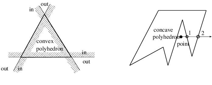
As shown in Figure 22.22, let us cast a half line from the tested point and count the number of intersections with the faces of the polyhedron (the calculation of these intersections is discussed in Section 22.6). If the result is an odd number, then the point is inside, otherwise it is outside. Because of numerical inaccuracies we might have difficulties to count the number of intersections when the half line is close to the edges. In such cases, the simplest solution is to find another half line and carry out the test with that.
The methods proposed to test the point in polyhedron can also be used for polygons limiting the space to the two-dimensional plane. For example, a point is in a general polygon if the half line originating at this point and lying in the plane of the polygon intersects the edges of the polygon odd times.
In addition to those methods, containment in convex polygons can be tested by adding the angles subtended by the edges from the point. If the sum is 360 degrees, then the point is inside, otherwise it is outside. For convex polygons, we can also test whether the point is on the same side of the edges as the polygon itself. This algorithm is examined in details for a particularly important special case, when the polygon is a triangle.
Let us consider a triangle of vertices  and
and  , and point
  lying in the plane of the triangle. The point is inside the triangle if and only if it is on the same side of the boundary lines as the third vertex. Note that cross product
  has a different direction for point
  lying on the different sides of oriented line
  , thus the direction of this vector can be used to classify points (should point
  be on line
  , the result of the cross product is zero). During classification the direction of
 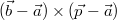 is compared to the direction of vector
  where tested point
  is replaced by third vertex
  . Note that vector
  happens to be the normal vector of the triangle plane (Figure 22.23).
We can determine whether two vectors have the same direction (their angle is zero) or they have opposite directions (their angle is 180 degrees) by computing their scalar product and looking at the sign of the result. The scalar product of vectors of similar directions is positive. Thus if scalar product  is positive, then point
  is on the same side of oriented line
  as
as  . On the other hand, if this scalar product is negative, then
  and
and  are on the opposite sides. Finally, if the result is zero, then point
  is on line
  . Point
  is inside the triangle if and only if all the following three conditions are met:
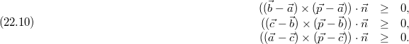
This test is robust since it gives correct result even if – due to numerical precision problems – point  is not exactly in the plane of the triangle as long as point
  is in the prism obtained by perpendicularly extruding the triangle from the plane.
Figure 22.23. Point in triangle containment test. The figure shows that case when point is on the left of oriented lines and , and on the right of line , that is, when it is not inside the triangle.
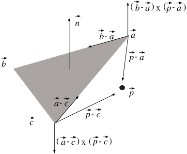
The evaluation of the test can be speeded up if we work in a two-dimensional projection plane instead of the three-dimensional space. Let us project point  as well as the triangle onto one of the coordinate planes. In order to increase numerical precision, that coordinate plane should be selected on which the area of the projected triangle is maximal. Let us denote the Cartesian coordinates of the normal vector by
  . If
. If  has the maximum absolute value, then the projection of the maximum area is on coordinate plane
  . If
. If  or
or  had the maximum absolute value, then planes
  or
or  would be the right choice. Here only the case of maximum
  is discussed.
Figure 22.24. Point in triangle containment test on coordinate plane . Third vertex can be either on the left or on the right side of oriented line , which can always be traced back to the case of being on the left side by exchanging the vertices.
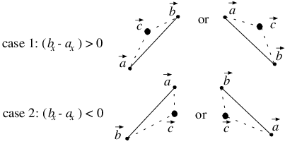
First the order of vertices are changed in a way that when travelling from vertex  to vertex
  , vertex
  is on the left side. Let us examine the equation of line
  :
:
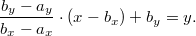
According to Figure 22.24 point  is on the left of the line if
  is above the line at
  :
:

Multiplying both sides by ( ), we get:

In the second case the denominator of the slope of the line is negative. Point  is on the left of the line if
  is below the line at
  :
:
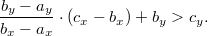
When the inequality is multiplied with negative denominator ( ), the relation is inverted:

Note that in both cases we obtained the same condition. If this condition is not met, then point  is not on the left of line
  , but is on the right. Exchanging vertices
  and
and  in this case, we can guarantee that
  will be on the left of the new line
  . It is also important to note that consequently point
  will be on the left of line
  and point
  will be on the left of line
  .
.
In the second step the algorithm tests whether point  is on the left with respect to all three boundary lines since this is the necessary and sufficient condition of being inside the triangle:

Two polyhedra collide when a vertex of one of them meets a face of the other, and if they are not bounced off, the vertex goes into the internal part of the other object (Figure 22.25). This case can be recognized with the discussed containment test. All vertices of one polyhedron is tested for containment against the other polyhedron. Then the roles of the two polyhedra are exchanged.
Figure 22.25. Polyhedron-polyhedron collision detection. Only a part of collision cases can be recognized by testing the containment of the vertices of one object with respect to the other object. Collision can also occur when only edges meet, but vertices do not penetrate to the other object.
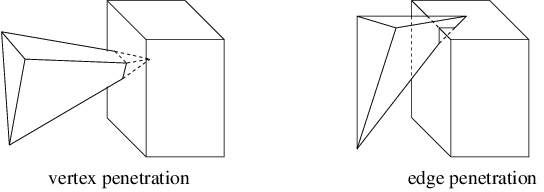
Apart from the collision between vertices and faces, two edges may also meet without vertex penetration (Figure 22.25). In order to recognize this edge penetration case, all edges of one polyhedron are tested against all faces of the other polyhedron. The test for an edge and a face is started by checking whether or not the two endpoints of the edge are on opposite sides of the plane, using inequality (22.9). If they are, then the intersection of the edge and the plane is calculated, and finally it is decided whether the face contains the intersection point.
Polyhedra collision detection tests each edge of one polyhedron against each face of the other polyhedron, which results in an algorithm of quadratic time complexity with respect to the number of vertices of the polyhedra. Fortunately, the algorithm can be speeded up applying bounding volumes (Subsection 22.6.2). Let us assign a simple bounding object to each polyhedron. Popular choices for bounding volumes are the sphere and the box. During testing the collision of two objects, first their bounding volumes are examined. If the two bounding volumes do not collide, then neither can the contained polyhedra collide. If the bounding volumes penetrate each other, then one polyhedra is tested against the other bounding volume. If this test is also positive, then finally the two polyhedra are tested. However, this last test is rarely required, and most of the collision cases can be solved by bounding volumes.
Clipping takes an object defining the clipping region and removes those points from another object which are outside the clipping region. Clipping may alter the type of the object, which cannot be specified by a similar equation after clipping. To avoid this, we allow only those kinds of clipping regions and objects where the object type is not changed by clipping. Let us assume that the clipping region is a half space or a polyhedron, while the object to be clipped is a point, a line segment or a polygon.
If the object to be clipped is a point, then containment can be tested with the algorithms of the previous subsection. Based on the result of the containment test, the point is either removed or preserved.
Let us consider a line segment of endpoints  and
and  , and of equation
  , (
, ( ), and a half plane defined by the following equation derived from equation (22.1):

Three cases need to be distinguished:
-
If both endpoints of the line segment are in the half space, then all points of the line segment are inside, thus the whole segment is preserved.
-
If both endpoints are out of the half space, then all points of the line segment are out, thus the line segment should be completely removed.
-
If one of the endpoints is out, while the other is in, then the endpoint being out should be replaced by the intersection point of the line segment and the boundary plane of the half space. The intersection point can be calculated by substituting the equation of the line segment into the equation of the boundary plane and solving the resulting equation for the unknown parameter:
Substituting parameter
 into the equation of the line segment, the coordinates of the intersection point can also be obtained.

This clipping algorithm tests first whether a vertex is inside or not. If the vertex is in, then it is also the vertex of the resulting polygon. However, if it is out, it can be ignored. On the other hand, the resulting polygon may have vertices other than the vertices of the original polygon. These new vertices are the intersections of the edges and the boundary plane of the half space. Such intersection occurs when one endpoint is in, but the other is out. While we are testing the vertices one by one, we should also check whether or not the next vertex is on the same side as the current vertex (Figure 22.26).
Figure 22.26. Clipping of simple convex polygon results in polygon . The vertices of the resulting polygon are the inner vertices of the original polygon and the intersections of the edges and the boundary plane.
![Clipping of simple convex polygon \vec{p}[0],\ldots,\vec{p}[5] results in polygon \vec{q}[0],\ldots,\vec{q}[4] . The vertices of the resulting polygon are the inner vertices of the original polygon and the intersections of the edges and the boundary plane.](images/view8Eng.png)
Suppose that the vertices of the polygon to be clipped are given in array  , and the vertices of the clipped polygon is expected in array
 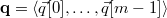 . The number of the vertices of the resulting polygon is stored in variable
  . Note that the vertex followed by the
  th vertex has usually index (
 ), but not in the case of the last,
  th vertex, which is followed by vertex
  . Handling the last vertex as a special case is often inconvenient. This can be eliminated by extending input array
  by new element
  , which holds the element of index 0 once again.
Using these assumptions, the Sutherland-Hodgeman polygon clipping algorithm:
Sutherland-Hodgeman-Polygon-Clipping(
)
12
FOR
TO3
DOIFis inside 4
THEN
The
th vertex is the vertex
of the resulting polygon. 5
6
IFis outside 7
THENEdge-Plane-Intersection()89
ELSEIFis inside 10
THENEdge-Plane-Intersection()1112
RETURN


Let us apply this algorithm for such a concave polygon which is expected to fall to several pieces during clipping (Figure 22.27). The algorithm storing the polygon in a single array is not able to separate the pieces and introduces even number of edges at parts where no edge could show up.
Figure 22.27. When concave polygons are clipped, the parts that should fall apart are connected by even number of edges.
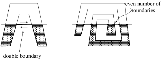
These even number of extra edges, however, pose no problems if the interior of the polygon is defined as follows: a point is inside the polygon if and only if starting a half line from here, the boundary polyline is intersected by odd number of times.
The presented algorithm is also suitable for clipping multiple connected polygons if the algorithm is executed separately for each closed polyline of the boundary.
As stated, a convex polyhedron can be obtained as the intersection of the half spaces defined by the planes of the polyhedron faces (left of Figure 22.22). It means that clipping on a convex polyhedron can be traced back to a series of clipping steps on half spaces. The result of one clipping step on a half plane is the input of clipping on the next half space. The final result is the output of the clipping on the last half space.
Axis aligned bounding boxes, abbreviated as AABBs, play an important role in image synthesis.
Definition 22.11 A box aligned parallel to the coordinate axes is called AABB. An AABB is specified with the minimum and maximum Cartesian coordinates:  .
.
Although when an object is clipped on an AABB, the general algorithms that clip on a convex polyhedron could also be used, the importance of AABBs is acknowledged by developing algorithms specially tuned for this case.
When a line segment is clipped to a polyhedron, the algorithm would test the line segment with the plane of each face, and the calculated intersection points may turn out to be unnecessary later. We should thus find an appropriate order of planes which makes the number of unnecessary intersection calculations minimal. A simple method that implements this idea is the Cohen-Sutherland line clipping algorithm.
Let us assign code bit 1 to a point that is outside with respect to a clipping plane, and code bit 0 if the point is inside with respect to this plane. Since an AABB has 6 sides, we get 6 bits forming a 6-bit code word (Figure 22.28). The interpretation of code bits  is the following:


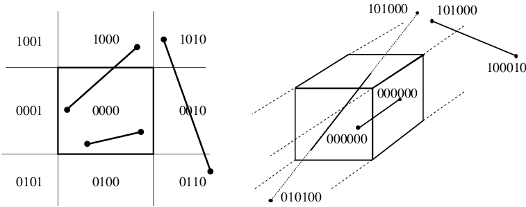
Points of code word 000000 are obviously inside, points of other code words are outside (Figure 22.28). Let the code words of the two endpoints of the line segment be  and
and  , respectively. If both of them are zero, then both endpoints are inside, thus the line segment is completely inside (trivial accept). If the two code words contain bit 1 at the same location, then none of the endpoints are inside with respect to the plane associated with this code bit. This means that the complete line segment is outside with respect to this plane, and can be rejected (trivial reject). This examination can be executed by applying the bitwise AND operation on code words
  and
and  (with the notations of the C programming language
  ), and checking whether or not the result is zero. If it is not zero, there is a bit where both code words have value 1.
Finally, if none of the two trivial cases hold, then there must be a bit which is 0 in one code word and 1 in the other. This means that one endpoint is inside and the other is outside with respect to the plane corresponding to this bit. The line segment should be clipped on this plane. Then the same procedure should be repeated starting with the evaluation of the code bits. The procedure is terminated when the conditions of either the trivial accept or the trivial reject are met.
The Cohen-Sutherland line clipping algorithm returns the endpoints of the clipped line by modifying the original vertices and indicates with TRUE return value if the line is not completely rejected:
Cohen-Sutherland-Line-Clipping(
)
1codeword of

Code bits by checking the inequalities. 2
codeword of
3
WHILETRUE4DOIFAND
5
THENRETURNTRUETrivial accept: inner line segment exists. 6
IF7
THENRETURNFALSETrivial reject: no inner line segment exists. 8
index of the first bit where
and
differ 9
intersection of line segment (
,
) and the plane of index
10
codeword of
11
IF12
THEN13


is outside w.r.t. plane
. 14
ELSE15


is outside w.r.t. plane
.
Exercises
22.4-1 Propose approaches to reduce the quadratic complexity of polyhedron-polyhedron collision detection.
22.4-2 Develop a containment test to check whether a point is in a CSG-tree.
22.4-3 Develop an algorithm clipping one polygon onto a concave polygon.
22.4-4 Find an algorithm computing the bounding sphere and the bounding AABB of a polyhedron.
22.4-5 Develop an algorithm that tests the collision of two triangles in the plane.
22.4-6 Generalize the Cohen-Sutherland line clipping algorithm to convex polyhedron clipping region.
22.4-7 Propose a method for clipping a line segment on a sphere.
Objects in the virtual world may move, get distorted, grow or shrink, that is, their equations may also depend on time. To describe dynamic geometry, we usually apply two functions. The first function selects those points of space, which belong to the object in its reference state. The second function maps these points onto points defining the object in an arbitrary time instance. Functions mapping the space onto itself are called transformations. A transformation maps point  to point
  . If the transformation is invertible, we can also find the original for some transformed point
  using inverse transformation
  .
.
If the object is defined in its reference state by inequality  , then the points of the transformed object are
since the originals belong to the set of points of the reference state.
Parametric equations define the Cartesian coordinates of the points directly. Thus the transformation of parametric surface  requires the transformations of its points
Similarly, the transformation of curve  is:
is:
Transformation  may change the type of object in the general case. It can happen, for example, that a simple triangle or a sphere becomes a complicated shape, which are hard to describe and handle. Thus it is worth limiting the set of allowed transformations. Transformations mapping planes onto planes, lines onto lines and points onto points are particularly important. In the next subsection we consider the class of homogeneous linear transformations, which meet this requirement.
So far the construction of the virtual world has been discussed using the means of the Euclidean geometry, which gave us many important concepts such as distance, parallelism, angle, etc. However, when the transformations are discussed in details, many of these concepts are unimportant, and can cause confusion. For example, parallelism is a relationship of two lines which can lead to singularities when the intersection of two lines is considered. Therefore, transformations are discussed in the context of another framework, called projective geometry.
The axioms of projective geometry turn around the problem of parallel lines by ignoring the concept of parallelism altogether, and state that two different lines always have an intersection. To cope with this requirement, every line is extended by a “point at infinity” such that two lines have the same extra point if and only if the two lines are parallel. The extra point is called the ideal point. The projective space contains the points of the Euclidean space (these are the so called affine points) and the ideal points. An ideal point “glues” the “ends” of an Euclidean line, making it topologically similar to a circle. Projective geometry preserves that axiom of the Euclidean geometry which states that two points define a line. In order to make it valid for ideal points as well, the set of lines of the Euclidean space is extended by a new line containing the ideal points. This new line is called the ideal line. Since the ideal points of two lines are the same if and only if the two lines are parallel, the ideal lines of two planes are the same if and only if the two planes are parallel. Ideal lines are on the ideal plane, which is added to the set of planes of the Euclidean space. Having made these extensions, no distinction is needed between the affine and ideal points. They are equal members of the projective space.
Introducing analytic geometry we noted that everything should be described by numbers in computer graphics. Cartesian coordinates used so far are in one to one relationship with the points of Euclidean space, thus they are inappropriate to describe the points of the projective space. For the projective plane and space, we need a different algebraic base.
Let us consider first the projective plane and find a method to describe its points by numbers. To start, a Cartesian coordinate system  is set up in this plane. Simultaneously, another Cartesian system
  is established in the three-dimensional space embedding the plane in a way that axes
  are parallel to axes
  , the plane is perpendicular to axis
  , the origin of the Cartesian system of the plane is in point
  of the three-dimensional space, and the points of the plane satisfy equation
  . The projective plane is thus embedded into a three-dimensional Euclidean space where points are defined by Descartes-coordinates (Figure 22.29). To describe a point of the projective plane by numbers, a correspondence is found between the points of the projective plane and the points of the embedding Euclidean space. An appropriate correspondence assigns that line of the Euclidean space to either affine or ideal point
  of the projective plane, which is defined by the origin of the coordinate system of the space and point
  .
.
Points of an Euclidean line that crosses the origin can be defined by parametric equation 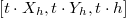 where
where  is a free real parameter. If point
  is an affine point of the projective plane, then the corresponding line is not parallel with plane
  (i.e.
(i.e.  is not constant zero). Such line intersects the plane of equation
  at point
 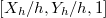 , thus the Cartesian coordinates of point
  in planar coordinate system
  are
are  . On the other hand, if point
  is ideal, then the corresponding line is parallel to the plane of equation
  (i.e.
(i.e.  ). The direction of the ideal point is given by vector
  .
.
Figure 22.29. The embedded model of the projective plane: the projective plane is embedded into a three-dimensional Euclidean space, and a correspondence is established between points of the projective plane and lines of the embedding three-dimensional Euclidean space by fitting the line to the origin of the three-dimensional space and the given point.
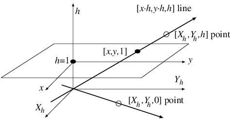
The presented approach assigns three dimensional lines crossing the origin and eventually  triplets to both the affine and the ideal points of the projective plane. These triplets are called the homogeneous coordinates of a point in the projective plane. Homogeneous coordinates are enclosed by brackets to distinguish them from Cartesian coordinates.
A three-dimensional line crossing the origin and describing a point of the projective plane can be defined by its arbitrary point except the origin. Consequently, all three homogeneous coordinates cannot be simultaneously zero, and homogeneous coordinates can be freely multiplied by the same non-zero scalar without changing the described point. This property justifies the name “homogeneous”.
It is often convenient to select that triplet from the homogeneous coordinates of an affine point, where the third homogeneous coordinate is 1 since in this case the first two homogeneous coordinates are identical to the Cartesian coordinates:

From another point of view, Cartesian coordinates of an affine point can be converted to homogeneous coordinates by extending the pair by a third element of value 1.
The embedded model also provides means to define the equations of the lines and line segments of the projective space. Let us select two different points on the projective plane and specify their homogeneous coordinates. The two points are different if homogeneous coordinates  of the first point cannot be obtained as a scalar multiple of homogeneous coordinates
  of the other point. In the embedding space, triplet
  can be regarded as Cartesian coordinates, thus the equation of the line fitted to points
  and
and  is:
is:
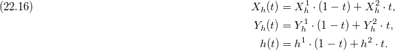
If  , then the affine points of the projective plane can be obtained by projecting the three-dimensional space onto the plane of equation
  . Requiring the two points be different, we excluded the case when the line would be projected to a single point. Hence projection maps lines to lines. Thus the presented equation really identifies the homogeneous coordinates defining the points of the line. If
  , then the equation expresses the ideal point of the line.
If parameter  has an arbitrary real value, then the points of a line are defined. If parameter
  is restricted to interval
  , then we obtain the line segment defined by the two endpoints.
We could apply the same method to introduce homogeneous coordinates of the projective space as we used to define the homogeneous coordinates of the projective plane, but this approach would require the embedding of the three-dimensional projective space into a four-dimensional Euclidean space, which is not intuitive. We would rather discuss another construction, which works in arbitrary dimensions. In this construction, a point is described as the centre of mass of a mechanical system. To identify a point, let us place weight  at reference point
  , weight
  at reference point
  , weight
  at reference point
  , and weight
  at reference point
  . The centre of mass of this mechanical system is:
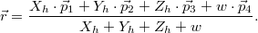
Let us denote the total weight by  . By definition, elements of quadruple
  are the homogeneous coordinates of the centre of mass.
To find the correspondence between homogeneous and Cartesian coordinates, the relationship of the two coordinate systems (the relationship of the basis vectors and the origin of the Cartesian coordinate system and of the reference points of the homogeneous coordinate system) must be established. Let us assume, for example, that the reference points of the homogeneous coordinate system are in points (1,0,0), (0,1,0), (0,0,1), and (0,0,0) of the Cartesian coordinate system. The centre of mass (assuming that total weight  is not zero) is expressed in Cartesian coordinates as follows:

Hence the correspondence between homogeneous coordinates  and Cartesian coordinates
  is (
is ( ):
):

The equations of lines in the projective space can be obtained either deriving them from the embedding four-dimensional Cartesian space, or using the centre of mass analogy:
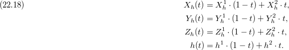
If parameter  is restricted to interval
  , then we obtain the equation of the projective line segment.
To find the equation of the projective plane, the equation of the Euclidean plane is considered (equation 22.1). The Cartesian coordinates of the points on an Euclidean plane satisfy the following implicit equation

Using the correspondence between the Cartesian and homogeneous coordinates (equation 22.17) we still describe the points of the Euclidean plane but now with homogeneous coordinates:
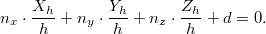
Let us multiply both sides of this equation by  , and add those points to the plane which have
  coordinate and satisfy this equation. With this step the set of points of the Euclidean plane is extended with the ideal points, that is, we obtained the set of points belonging to the projective plane. Hence the equation of the projective plane is a homogeneous linear equation:

or in matrix form:
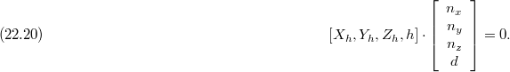
Note that points and planes are described by row and column vectors, respectively. Both the quadruples of points and the quadruples of planes have the homogeneous property, that is, they can be multiplied by non-zero scalars without altering the solutions of the equation.
Transformations defined as the multiplication of the homogeneous coordinate vector of a point by a constant 
 matrix are called homogeneous linear transformations:

Theorem 22.12 Homogeneous linear transformations map points to points.
Proof. A point can be defined by homogeneous coordinates in form  , where
  is an arbitrary, non-zero constant. The transformation results in
  when a point is transformed, which are the
  -multiples of the same vector, thus the result is a single point in homogeneous coordinates.
Note that due to the homogeneous property, homogeneous transformation matrix  is not unambiguous, but can be freely multiplied by non-zero scalars without modifying the realized mapping.
Theorem 22.13 Invertible homogeneous linear transformations map lines to lines.
Proof. Let us consider the parametric equation of a line:

and transform the points of this line by multiplying the quadruples with the transformation matrix:


where  and
and  are the transformations of
  and
and  , respectively. Since the transformation is invertible, the two points are different. The resulting equation is the equation of a line fitted to the transformed points.
We note that if we had not required the invertibility of the the transformation, then it could have happened that the transformation would have mapped the two points to the same point, thus the line would have degenerated to single point.
If parameter  is limited to interval
  , then we obtain the equation of the projective line segment, thus we can also state that a homogeneous linear transformation maps a line segment to a line segment. Even more generally, a homogeneous linear transformation maps convex combinations to convex combinations. For example, triangles are also mapped to triangles.
However, we have to be careful when we try to apply this theorem in the Euclidean plane or space. Let us consider a line segment as an example. If coordinate  has different sign at the two endpoints, then the line segment contains an ideal point. Such projective line segment can be intuitively imagined as two half lines and an ideal point sticking the “endpoints” of these half lines at infinity, that is, such line segment is the complement of the line segment we are accustomed to. It may happen that before the transformation, coordinates
  of the endpoints have similar sign, that is, the line segment meets our intuitive image about Euclidean line segments, but after the transformation, coordinates
  of the endpoints will have different sign. Thus the transformation wraps around our line segment.
Theorem 22.14 Invertible homogeneous linear transformations map planes to planes.
Proof. The originals of transformed points 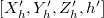 defined by
  are on a plane, thus satisfy the original equation of the plane:
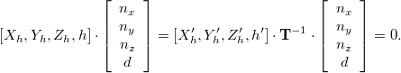
Due to the associativity of matrix multiplication, the transformed points also satisfy equation
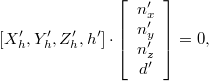
which is also a plane equation, where
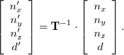
This result can be used to obtain the normal vector of a transformed plane.
An important subclass of homogeneous linear transformations is the set of affine transformations, where the Cartesian coordinates of the transformed point are linear functions of the original Cartesian coordinates:
where vector  describes translation,
  is a matrix of size
  and expresses rotation, scaling, mirroring, etc., and their arbitrary combination. For example, the rotation around axis
  , (
, ( ) by angle
  is given by the following matrix

This expression is known as the Rodrigues-formula.
Affine transformations map the Euclidean space onto itself, and transform parallel lines to parallel lines. Affine transformations are also homogeneous linear transformations since equation (22.22) can also be given as a  matrix operation, having changed the Cartesian coordinates to homogeneous coordinates by adding a fourth coordinate of value 1:
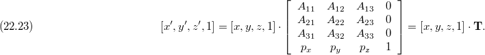
A further specialization of affine transformations is the set of congruence transformations (isometries) which are distance and angle preserving.
Theorem 22.15 In a congruence transformation the rows of matrix  have unit length and are orthogonal to each other.
Proof. Let us use the property that a congruence is distance and angle preserving for the case when the origin and the basis vectors of the Cartesian system are transformed. The transformation assigns point  to the origin and points
  ,
,  , and
, and  to points
  ,
,  , and
, and  , respectively. Because the distance is preserved, the distances between the new points and the new origin are still 1, thus
  ,
,  , and
, and  . On the other hand, because the angle is also preserved, vectors
  ,
,  , and
, and  are also perpendicular to each other.
Exercises
22.5-1 Using the Cartesian coordinate system as an algebraic basis, prove the axioms of the Euclidean geometry, for example, that two points define a line, and that two different lines may intersect each other at most at one point.
22.5-2 Using the homogeneous coordinates as an algebraic basis, prove an axiom of the projective geometry stating that two different lines intersect each other in exactly one point.
22.5-3 Prove that homogeneous linear transformations map line segments to line segments using the centre of mass analogy.
22.5-4 How does an affine transformation modify the volume of an object?
22.5-5 Give the matrix of that homogeneous linear transformation which translates by vector  .
.
22.5-6 Prove the Rodrigues-formula.
22.5-7 A solid defined by inequality  in time
  moves with uniform constant velocity
  . Let us find the inequality of the solid at an arbitrary time instance
  .
.
22.5-8 Prove that if the rows of matrix  are of unit length and are perpendicular to each other, then the affine transformation is a congruence. Show that for such matrices
  .
.
22.5-9 Give that homogeneous linear transformation which projects the space from point  onto a plane of normal
  and place vector
  .
.
22.5-10 Show that five point correspondences unambiguously identify a homogeneous linear transformation if no four points are co-planar.
When a virtual world is rendered, we have to identify the surfaces visible in different directions from the virtual eye. The set of possible directions is defined by a rectangle shaped window which is decomposed to a grid corresponding to the pixels of the screen (Figure 22.30). Since a pixel has a unique colour, it is enough to solve the visibility problem in a single point of each pixel, for example, in the points corresponding to pixel centres.
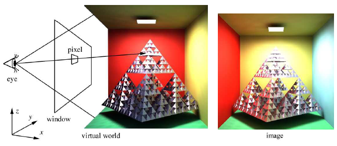
The surface visible at a direction from the eye can be identified by casting a half line, called ray, and identifying its intersection closest to the eye position. This operation is called ray tracing. Ray tracing has many applications. For example, shadow computation tests whether or not a point is occluded from the light source, which requires a ray to be sent from the point at the direction of the light source and the determination whether this ray intersects any surface closer than the light source. Ray tracing is also used by collision detection since a point moving with constant and uniform speed collides that surface which is first intersected by the ray describing the motion of the point.
A ray is defined by the following equation:

where  is the place vector of the ray origin,
  is the direction of the ray, and ray parameter
  characterizes the distance from the origin. Let us suppose that direction vector
  has unit length. In this case parameter
  is the real distance, otherwise it would only be proportional to the distance.
Footnote. In collision detection  is not a unit vector, but the velocity of the moving point since this makes ray parameter
  express the collision time.
If parameter  is negative, then the point is behind the eye and is obviously not visible. The identification of the closest intersection with the ray means the determination of the intersection point having the smallest, positive ray parameter. In order to find the closest intersection, the intersection calculation is tried with each surface, and the closest is retained. This algorithm obtaining the first intersection is:
Ray-First-Intersection(
)
1
Initialization to the maximum size in the virtual world. 2
FOReach object3
DORay-Surface-Intersection()Negative if no intersection exists. 4
IF
Is the new intersection closer? 5
THEN
Ray parameter of the closest intersection so far. 6

Closest object so far. 7
IF
THENHas been intersection at all? 8
THEN
Intersection point using the ray equation. 9
RETURN10
ELSERETURN“no intersection”No intersection.


This algorithm inputs the ray defined by origin  and direction
  , and outputs the ray parameter of the intersection in variable
  , the intersection point in
  , and the visible object in
  . The algorithm calls function
 Ray-Surface-Intersection for each object, which determines the intersection of the ray and the given object, and indicates with a negative return value if no intersection exists. Function Ray-Surface-Intersection should be implemented separately for each surface type.
The identification of the intersection between a ray and a surface requires the solution of an equation. The intersection point is both on the ray and on the surface, thus it can be obtained by inserting the ray equation into the equation of the surface and solving the resulting equation for the unknown ray parameter.
For implicit surfaces of equation  , the intersection can be calculated by solving the following scalar equation for
  :
: 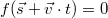 .
.
Let us take the example of quadrics that include the sphere, the ellipsoid, the cylinder, the cone, the paraboloid, etc. The implicit equation of a general quadric contains a quadratic form:
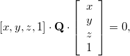
where  is a
is a  matrix. Substituting the ray equation into the equation of the surface, we obtain
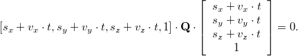
Rearranging the terms, we get a second order equation for unknown parameter  :
:

where  and
and  .
.
This equation can be solved using the solution formula of second order equations. Now we are interested in only the real and positive roots. If two such roots exist, then the smaller one corresponds to the intersection closer to the origin of the ray.
The intersection of parametric surface  and the ray is calculated by first solving the following equation for unknown parameters
then checking whether or not  is positive and parameters
  are inside the allowed parameter range of the surface.
Roots of non-linear equations are usually found by numeric methods. On the other hand, the surface can also be approximated by a triangle mesh, which is intersected by the ray. Having obtained the intersection on the coarse mesh, the mesh around this point is refined, and the intersection calculation is repeated with the refined mesh.
To compute the ray intersection for a triangle of vertices  ,
,  , and
, and  , first the ray intersection with the plane of the triangle is found. Then it is decided whether or not the intersection point with the plane is inside the triangle. The normal and a place vector of the triangle plane are
  , and
, and  , respectively, thus points
  of the plane satisfy the following equation:

The intersection of the ray and this plane is obtained by substituting the ray equation (equation (22.24)) into this plane equation, and solving it for unknown parameter  . If root
  is positive, then it is inserted into the ray equation to get the intersection point with the plane. However, if the root is negative, then the intersection is behind the origin of the ray, thus is invalid. Having a valid intersection with the plane of the triangle, we check whether this point is inside the triangle. This is a containment problem, which is discussed in Subsection 22.4.1.
The surface of an AABB, that is an axis aligned block, can be subdivided to 6 rectangular faces, or alternatively to 12 triangles, thus its intersection can be solved by the algorithms discussed in the previous subsections. However, realizing that in this special case the three coordinates can be handled separately, we can develop more efficient approaches. In fact, an AABB is the intersection of an  -stratum defined by inequality
  , a
, a  -stratum defined by
  and a
and a  -stratum of inequality
  . For example, the ray parameters of the intersections with the
  -stratum are:
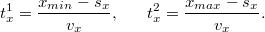
The smaller of the two parameter values corresponds to the entry at the stratum, while the greater to the exit. Let us denote the ray parameter of the entry by  , and the ray parameter of the exit by
  . The ray is inside the
  -stratum while the ray parameter is in
  . Repeating the same calculation for the
  and
and  -strata as well, three ray parameter intervals are obtained. The intersection of these intervals determine when the ray is inside the AABB. If parameter
  obtained as the result of intersecting the strata is negative, then the AABB is behind the eye, thus no ray–AABB intersection is possible. If only
  is negative, then the ray starts at an internal point of the AABB, and the first intersection is at
  . Finally, if
  is positive, then the ray enters the AABB from outside at parameter
  .
.
The computation of the unnecessary intersection points can be reduced by applying the Cohen – Sutherland line clipping algorithm (subsection 22.4.3). First, the ray is replaced by a line segment where one endpoint is the origin of the ray, and the other endpoint is an arbitrary point on the ray which is farther from the origin than any object of the virtual world. Then this line segment is tried to be clipped by the AABB. If the Cohen – Sutherland algorithm reports that the line segment has no internal part, then the ray has no intersection with the AABB.
A naive ray tracing algorithm tests each object for a ray to find the closest intersection. If there are  objects in the space, the running time of the algorithm is
  both in the average and in the worst case. The storage requirement is also linear in terms of the number of objects.
The method would be speeded up if we could exclude certain objects from the intersection test without testing them one by one. The reasons of such exclusion include that these objects are “behind” the ray or “not in the direction of the ray”. Additionally, the speed is also expected to improve if we can terminate the search having found an intersection supposing that even if other intersections exist, they are surely farther than the just found intersection point. To make such decisions safely, we need to know the arrangement of objects in the virtual world. This information is gathered during the pre-processing phase. Of course, pre-processing has its own computational cost, which is worth spending if we have to trace a lot of rays.
One of the simplest ray tracing acceleration technique uses bounding volumes, The bounding volume is a shape of simple geometry, typically a sphere or an AABB, which completely contains a complex object. When a ray is traced, first the bounding volume is tried to be intersected. If there is no intersection with the bounding volume, then neither can the contained object be intersected, thus the computation time of the ray intersection with the complex object is saved. The bounding volume should be selected in a way that the ray intersection is computationally cheap, and it is a tight container of the complex object.
The application of bounding volumes does not alter the linear time complexity of the naive ray tracing. However, it can increase the speed by a scalar factor.
On the other hand, bounding volumes can also be organized in a hierarchy putting bounding volumes inside bigger bounding volumes recursively. In this case the ray tracing algorithm traverses this hierarchy, which is possible in sub-linear time.
Let us find the AABB of the complete virtual world and subdivide it by an axis aligned uniform grid of cell sizes  (Figure 22.31).
Figure 22.31. Partitioning the virtual world by a uniform grid. The intersections of the ray and the coordinate planes of the grid are at regular distances , , and , respectively.
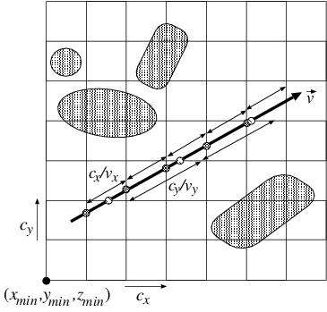
In the preprocessing phase, for each cell we identify those objects that are at least partially contained by the cell. The test of an object against a cell can be performed using a clipping algorithm (subsection 22.4.3), or simply checking whether the cell and the AABB of the object overlap.
Uniform-Grid-Construction()
1 Compute the minimum corner of the AABB () and cell sizes
2
FOReach cell3
DOobject list of cellempty 4
FOReach object
Register objects overlapping
with this cell. 5
DOIFcelland the AABB of object
overlap 6
THENadd objectto object list of cell

During ray tracing, cells intersected by the ray are visited in the order of their distance from the ray origin. When a cell is processed, only those objects need to be tested for intersection which overlap with this cell, that is, which are registered in this cell. On the other hand, if an intersection is found in the cell, then intersections belonging to other cells cannot be closer to the ray origin than the found intersection. Thus the cell marching can be terminated. Note that when an object registered in a cell is intersected by the ray, we should also check whether the intersection point is also in this cell.
We might meet an object again in other cells. The number of ray–surface intersection can be reduced if the results of ray–surface intersections are stored with the objects and are reused when needed again.
As long as no ray–surface intersection is found, the algorithm traverses those cells which are intersected by the ray. Indices  of the first cell are computed from ray origin
  , minimum corner
  of the grid, and sizes
  of the cells:
Uniform-Grid-Enclosing-Cell(
)
1Integer()2Integer()3Integer()4RETURN


The presented algorithm assumes that the origin of the ray is inside the subspace covered by the grid. Should this condition not be met, then the intersection of the ray and the scene AABB is computed, and the ray origin is moved to this point.
The initial values of ray parameters  are computed as the intersection of the ray and the coordinate planes by the
 Uniform-grid-ray-parameter-initialization algorithm:
Uniform-Grid-Ray-Parameter-Initialization(
)
1IF2
THEN3
ELSEIF4
THEN5
ELSE
The maximum distance. 6
IF7
THEN8
ELSEIF9
THEN10
ELSE11
IF12
THEN13
ELSEIF14
THEN15
ELSE16
RETURN
The next cell of the sequence of the visited cells is determined by the 3D line drawing algorithm (3DDDA algorithm). This algorithm exploits the fact that the ray parameters of the intersection points with planes perpendicular to axis  (and similarly to axes
  and
and  ) are regularly placed at distance
  (
( , and
, and  , respectively), thus the ray parameter of the next intersection can be obtained with a single addition (Figure 22.31). Ray parameters
  ,
,  , and
, and  are stored in global variables, and are incremented by constant values. The smallest from the three ray parameters of the coordinate planes identifies the next intersection with the cell.
The following algorithm computes indices  of the next intersected cell, and updates ray parameters
  :
:
Uniform-Grid-Next-Cell(
)
1IF
Next intersection is on the plane perpendicular to axis
. 2
THEN
Function
returns the sign. 3
4
ELSE IF
Next intersection is on the plane perpendicular to axis
. 5
THEN6
7
ELSE IF
Next intersection is on the plane perpendicular to axis
. 8
THEN9
To summarize, a complete ray tracing algorithm is presented, which exploits the uniform grid generated during preprocessing and computes the ray-surface intersection closest to the ray origin. The minimum of ray parameters  assigned to the coordinate planes, i.e. variable
  , determines the distance as far as the ray is inside the cell. This parameter is used to decide whether or not a ray-surface intersection is really inside the cell.
Ray-First-Intersection-with-Uniform-Grid(
)
1Uniform-Grid-Enclosing-Cell()2Uniform-Grid-Ray-Parameter-Initialization()3WHILEare inside the grid 4
DO
Here is the exit from the cell. 5

Initialization: no intersection yet. 6
FOReach objectregistered in cell (
) 7
DORay-Surface-Intersection()Negative: no intersection. 8
IF
Is the new intersection closer? 9
THEN
The ray parameter of the closest intersection so far. 10

The first intersected object. 11
IF
Was intersection in the cell? 12
THEN
The position of the intersection. 13
RETURN
Termination. 14
Uniform-Grid-Next-Cell()3DDDA. 15
RETURN“no intersection”


The preprocessing phase of the uniform grid algorithm tests each object with each cell, thus runs in  time where
  and
and  are the numbers of objects and cells, respectively. In practice, the resolution of the grid is set to make
  proportional to
  since in this case, the average number of objects per cell becomes independent of the total number of objects. Such resolution makes the preprocessing time quadratic, that is
  . We note that sorting objects before testing them against cells may reduce this complexity, but this optimization is not crucial since not the preprocessing but the ray tracing time is critical. Since in the worst case all objects may overlap with each cell, the storage space is also in
  .
.
The ray tracing time can be expressed by the following equation:

where  is the time needed to identify the cell containing the origin of the ray,
  is the number of ray–surface intersection tests until the first intersection is found,
  is the time required by a single ray–surface intersection test,
  is the number of visited cells, and
  is the time needed to step onto the next cell.
To find the first cell, the coordinates of the ray origin should be divided by the cell sizes, and the cell indices are obtained by rounding the results. This step thus runs in constant time. A single ray–surface intersection test also requires constant time. The next cell is determined by the 3DDDA algorithm in constant time as well. Thus the complexity of the algorithm depends only on the number of intersection tests and the number of the visited cells.
Considering a worst case scenario, a cell may contain all objects, requiring  intersection test with
  objects. In the worst case the ray tracing has linear complexity. This means that the uniform grid algorithm needs quadratic preprocessing time and storage, but solves the ray tracing problem still in linear time as the naive algorithm, which is quite disappointing. However, uniform grids are still worth using since worst case scenarios are very unlikely. The fact is that classic complexity measures describing the worst case characteristics are not appropriate to compare the naive algorithm and the uniform grid based ray tracing. For a reasonable comparison, the probabilistic analysis of the algorithms is needed.
To carry out the average case analysis, the scene model, i.e. the probability distribution of the possible virtual world models must be known. In practical situations, this probability distribution is not available, therefore it must be estimated. If the model of the virtual world were too complicated, we would not be able to analytically determine the average, i.e. the expected running time of the ray tracing algorithm. A simple, but also justifiable model is the following: Objects are spheres of the same radius  , and sphere centres are uniformly distributed in space.
Since we are interested in the asymptotic behavior when the number of objects is really high, uniform distribution in a finite space would not be feasible. On the other hand, the boundary of the space would pose problems. Thus, instead of dealing with a finite object space, the space should also be expanded as the number of objects grows to sustain constant average spatial object density. This is a classical method in probability theory, and its known result is the Poisson point process.
Definition 22.16 A Poisson point process  counts the number of points in subset
  of space in a way that
-
 is a Poisson distribution of parameter
  , where
  is a positive constant called “intensity” and
  is the volume of
  , thus the probability that
  contains exactly
  points is
 and the expected number of points in volume
 is
is  ;
; -
for disjoint
 sets random variables
  are independent.
Using the Poisson point process, the probabilistic model of the virtual world is:
-
The object space consists of spheres of the same radius
 .
. -
The sphere centres are the realizations of a Poisson point process of intensity
 .
.
Having constructed a probabilistic virtual world model, we can start the analysis of the candidate algorithms assuming that the rays are uniformly distributed in space.
Figure 22.32. Encapsulation of the intersection space by the cells of the data structure in a uniform subdivision scheme. The intersection space is a cylinder of radius . The candidate space is the union of those spheres that may overlap a cell intersected by the ray.
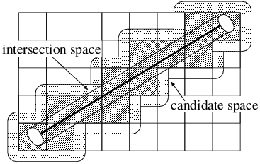
Looking at Figure 22.32 we can see a ray that passes through certain cells of the space partitioning data structure. The collection of those sphere centres where the sphere would have an intersection with a cell is called the candidate space associated with this cell.
Only those spheres of radius  can have intersection with the ray whose centres are in a cylinder of radius
  around the ray. This cylinder is called the intersection space (Figure 22.32). More precisely, the intersection space also includes two half spheres at the bottom and at the top of the cylinder, but these will be ignored.
As the ray tracing algorithm traverses the data structure, it examines each cell that is intersected by the ray. If the cell is empty, then the algorithm does nothing. If the cell is not empty, then it contains, at least partially, a sphere which is tried to be intersected. This intersection succeeds if the centre of the sphere is inside the intersection space and fails if it is outside.
The algorithm should try to intersect objects that are in the candidate space, but this intersection will be successful only if the object is also contained by the intersection space. The probability of the success  is the ratio of the projected areas of the intersection space and the candidate space associated with this cell.
From the probability of the successful intersection in a non-empty cell, the probability that the intersection is found in the first, second, etc. cells can also be computed. Assuming statistical independence, the probabilities that the first, second, third, etc. intersection is the first successful intersection are  ,
,  ,
,  , etc., respectively. This is a geometric distribution with expected value
  . Consequently, the expected number of the ray–object intersection tests is:

If the ray is parallel to one of the sides, then the projected size of the candidate space is  where
where  is the edge size of a cell and
  is the radius of the spheres. The other extreme case happens when the ray is parallel to the diagonal of the cubic cell, where the projection is a rounded hexagon having area
  . The success probability is then:
According to equation (22.27), the average number of intersection calculations is the reciprocal of this probability:

Note that if the size of the cell is equal to the diameter of the sphere ( ), then
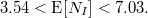
This result has been obtained assuming that the number of objects converges to infinity. The expected number of intersection tests, however, remains finite and relatively small.
In the following analysis the conditional expected value theorem will be used. An appropriate condition is the length of the ray segment between its origin and the closest intersection. Using its probability density  as a condition, the expected number of visited cells
  can be written in the following form:
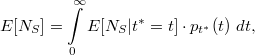
where  is the length of the ray and
  is its probability density.
Since the intersection space is a cylinder if we ignore the half spheres around the beginning and the end, its total volume is  . Thus the probability that intersection occurs before
  is:
is:
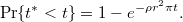
Note that this function is the cumulative probability distribution function of  . The probability density can be computed as its derivative, thus we obtain:
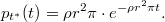
The expected length of the ray is then:

In order to simplify the analysis, we shall assume that the ray is parallel to one of the coordinate axes. Since all cells have the same edge size  , the number of cells intersected by a ray of length
  can be estimated as
  . This estimation is quite accurate. If the the ray is parallel to one of the coordinate axes, then the error is at most 1. In other cases the real value can be at most
  times the given estimation. The estimated expected number of visited cells is then:

For example, if the cell size is similar to the object size ( ), and the expected number of sphere centres in a cell is
  , then
  . Note that the expected number of visited cells is also constant even for infinite number of objects.
We concluded that the expected numbers of required intersection tests and visited cells are asymptotically constant, thus the expected time complexity of the uniform grid based ray tracing algorithm is constant after quadratic preprocessing time. The value of the running time can be controlled by cell size  according to equations (22.28) and (22.30). Smaller cell sizes reduce the average number of intersection tests, but increase the number of visited cells.
According to the probabilistic model, the average number of objects overlapping with a cell is also constant, thus the storage is proportional to the number of cells. Since the number of cells is set proportional to the number of objects, the expected storage complexity is also linear unlike the quadratic worst-case complexity.
The expected constant running time means that asymptotically the running time is independent of the number of objects, which explains the popularity of the uniform grid based ray tracing algorithm, and also the popularity of the algorithms presented in the next subsections.
Uniform grids require many unnecessary cell steps. For example, the empty spaces are not worth partitioning into cells, and two cells are worth separating only if they contain different objects. Adaptive space partitioning schemes are based on these recognitions. The space can be partitioned adaptively following a recursive approach. This results in a hierarchical data structure, which is usually a tree. The type of this tree is the base of the classification of such algorithms.
The adaptive scheme discussed in this subsection uses an octal tree (octree for short), where non-empty nodes have 8 children. An octree is constructed by the following algorithm:
-
For each object, an AABB is found, and object AABBs are enclosed by a scene AABB. The scene AABB is the cell corresponding to the root of the octree.
-
If the number of objects overlapping with the current cell exceeds a predefined threshold, then the cell is subdivided to 8 cells of the same size by halving the original cell along each coordinate axis. The 8 new cells are the children of the node corresponding to the original cell. The algorithm is recursively repeated for the child cells.
-
The recursive tree building procedure terminates if the depth of the tree becomes too big, or when the number of objects overlapping with a cell is smaller than the threshold.
The result of this construction is an octree (Figure 22.33). Overlapping objects are registered in the leaves of this tree.
When a ray is traced, those leaves of the tree should be traversed which are intersected by the ray, and ray–surface intersection test should be executed for objects registered in these leaves:
Ray-First-Intersection-with-Octree(
)
1intersection of the ray and the scene AABB 2
WHILEis inside of the scene AABB
Traversal of the tree. 3
Octree-Cell-Search()4ray parameter of the intersection of the
and the ray 5

Initialization: no ray–surface intersection yet. 6
FOReach objectregistered in
7
DORay-Surface-Intersection()Negative if no intersection exists. 8
IF
Is the new intersection closer? 9
THEN
Ray parameter of the closest intersection so far. 10

First intersected object so far. 11
IF
Has been intersection at all ? 12
THEN
Position of the intersection. 13
RETURN14
A point in the next cell. 15
RETURN“no intersection”


Figure 22.33. A quadtree partitioning the plane, whose three-dimensional version is the octree. The tree is constructed by halving the cells along all coordinate axes until a cell contains “just a few” objects, or the cell sizes gets smaller than a threshold. Objects are registered in the leaves of the tree.
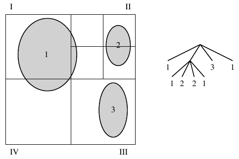
The identification of the next cell intersected by the ray is more complicated for octrees than for uniform grids. The Octree-Cell-Search algorithm determines that leaf cell which contains a given point. At each level of the tree, the coordinates of the point are compared to the coordinates of the centre of the cell. The results of these comparisons determine which child contains the point. Repeating this test recursively, we arrive at a leaf sooner or later.
In order to identify the next cell intersected by the ray, the intersection point of the ray and the current cell is computed. Then, ray parameter  of this intersection point is increased “a little” (this little value is denoted by
  in algorithm
 Ray-First-Intersection-with-Octree). The increased ray parameter is substituted into the ray equation, resulting in point  that is already in the next cell. The cell containing this point can be identified with
 Octree-cell-search.
Cells of the octree may be larger than the allowed minimal cell, therefore the octree algorithm requires less number of cell steps than the uniform grid algorithm working on the minimal cells. However, larger cells reduce the probability of the successful intersection tests since in a large cell it is less likely that a random ray intersecting the cell also intersects a contained object. Smaller successful intersection probability, on the other hand, results in greater expected number of intersection tests, which affects the performance negatively. It also means that non-empty octree cells are worth subdividing until the minimum cell size is reached even if the cell contains just a single object. Following this strategy, the size of the non-empty cells are similar, thus the results of the complexity analysis made for the uniform grid remain to be applicable to the octree as well. Since the probability of the successful intersection depends on the size of the non-empty cells, the expected number of needed intersection tests is still given by inequality (22.28). It also means that when the minimal cell size of an octree equals to the cell size of a uniform grid, then the expected number of intersection tests is equal in the two algorithms.
The advantage of the ocree is the ability to skip empty spaces, which reduces the number of cell steps. Its disadvantage is, however, that the time of the next cell identification is not constant. This identification requires the traversal of the tree. If the tree construction is terminated when a cell contains small number of objects, then the number of leaf cells is proportional to the number of objects. The depth of the tree is in  , so is the time needed to step onto the next cell.
An octree adapts to the distribution of the objects. However, the partitioning strategy of octrees always halves the cells without taking into account where the objects are, thus the adaptation is not perfect. Let us consider a partitioning scheme which splits a cell into two cells to make the tree balanced. Such method builds a binary tree which is called binary space partitioning tree, abbreviated as BSP-tree. If the separating plane is always perpendicular to one of the coordinate axes, then the tree is called kd-tree.
Figure 22.34. A kd-tree. A cell containing “many” objects are recursively subdivided to two cells with a plane that is perpendicular to one of the coordinate axes.
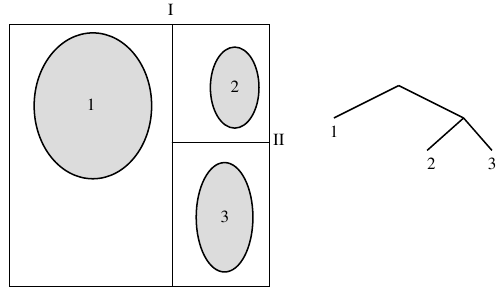
The separating plane of a kd-tree node can be placed in many different ways:
-
the spatial median method halves the cell into two congruent cells.
-
the object median method finds the separating plane to have the same number of objects in the two child cells.
-
the cost driven method estimates the average computation time needed when a cell is processed during ray tracing, and minimizes this value by placing the separating plane. An appropriate cost model suggests to separate the cell to make the probabilities of the ray–surface intersection of the two cells similar.
The probability of the ray–surface intersection can be computed using a fundamental theorem of the integral geometry:
Theorem 22.17 If convex solid  contains another convex solid
  , then the probability that a uniformly distributed line intersects solid
  provided that the line intersected
  equals to the ratio of the surface areas of objects
  and
and  .
.
According to this theorem the cost driven method finds the separating plane to equalize the surface areas in the two children.
Let us now present a general kd-tree construction algorithm. Parameter  identifies the current cell,
  is the current depth of recursion, and
  stores the orientation of the current separating plane. A
  is associated with its two children (
 and
and  ), and its left-lower-closer and right-upper-farther corners (
 and
and  ). Cells also store the list of those objects which overlap with the cell. The orientation of the separation plane is determined by a round-robin scheme implemented by function
 Round-robin providing a sequence like ( ). When the following recursive algorithm is called first, it gets the scene AABB in variable
  and the value of variable
  is zero:
Kd-Tree-Construction(
)
1IFthe number of objects overlapping withis small or
is large 2
THENRETURN3 AABB ofand AABB of
AABB of
4
IF5
THENperpendicular separating plane of
6
perpendicular separating plane of
7
ELSEIF8
THENperpendicular separating plane of
9
perpendicular separating plane of
10
ELSEIF11
THENperpendicular separating plane of
12
perpendicular separating plane of
13
FOReach objectof
14
DOIFobjectis in the AABB of
15
THENassign objectto the list of
16
IFobjectis in the AABB of
17
THENassign objectto the list of
18
Kd-Tree-Construction(, Round-Robin())19Kd-Tree-Construction(, Round-Robin())


Now we discuss an algorithm that traverses the constructed kd-tree and finds the visible object. First we have to test whether the origin of the ray is inside the scene AABB. If it is not, the intersection of the ray and the scene AABB is computed, and the origin of the ray is moved there. The identification of the cell containing the ray origin requires the traversal of the tree. During the traversal the coordinates of the point are compared to the coordinates of the separating plane. This comparison determines which child should be processed recursively until a leaf node is reached. If the leaf cell is not empty, then objects overlapping with the cell are intersected with the ray, and the intersection closest to the origin is retained. The closest intersection is tested to see whether or not it is inside the cell (since an object may overlap more than one cells, it can also happen that the intersection is in another cell). If the intersection is in the current cell, then the needed intersection has been found, and the algorithm can be terminated. If the cell is empty, or no intersection is found in the cell, then the algorithm should proceed with the next cell. To identify the next cell, the ray is intersected with the current cell identifying the ray parameter of the exit point. Then the ray parameter is increased “a little” to make sure that the increased ray parameter corresponds to a point in the next cell. The algorithm keeps repeating these steps as it processes the cells of the tree.
This method has the disadvantage that the cell search always starts at the root, which results in the repetitive traversals of the same nodes of the tree.
This disadvantage can be eliminated by putting the cells to be visited into a stack, and backtracking only to the point where a new branch should be followed. When the ray arrives at a node having two children, the algorithm decides the order of processing the two child nodes. Child nodes are classified as “near” and “far” depending on whether or not the child cell is on the same side of the separating plane as the origin of the ray. If the ray intersects only the ``near'' child, then the algorithm processes only that subtree which originates at this child. If the ray intersects both children, then the algorithm pushes the “far” node onto the stack and starts processing the “near” node. If no intersection exists in the “near” node, then the stack is popped to obtain the next node to be processed.
The notations of the ray tracing algorithm based on kd-tree traversal are shown by Figure 22.35. The algorithm is the following:
Ray-First-Intersection-with-kd-Tree(
)
1Ray-AABB-Intersection()Intersection with the scene AABB. 2
IFno intersection 3THENRETURN“no intersection” 4Push()5WHILEthe stack is not emptyVisit all nodes. 6
DOPop()7WHILEis not a leaf 8
DOorientation of the separating plane of the
9
10
Ray parameter of the separating plane. 11
IF
Is
on the left side of the separating plane? 12
THEN
Left. 13
ELSE
Right. 14
IFor
15
THEN
The ray intersects only the
cell. 16
ELSEIF17
THEN
The ray intersects only the
cell. 18
ELSEPush()The ray intersects both cells. 19

First
is intersected. 20

The ray exists at
from the
cell.
If the current cell is a leaf. 21

Maximum ray parameter in this cell. 22
FOReach objectof
23
DORay-surface-intersection()Negative if no intersection exists. 24
IF
Is the new intersection closer to the ray origin? 25
THEN
The ray parameter of the closest intersection so far. 26

The object intersected closest to the ray origin. 27
IF
Has been intersection at all in the cell? 28
THEN
The intersection point. 29
RETURN
Intersection has been found. 30
RETURN“no intersection”No intersection.


Figure 22.35. Notations and cases of algorithm Ray-First-Intersection-with-kd-Tree. , , and are the ray parameters of the entry, exit, and the separating plane, respectively. is the signed distance between the ray origin and the separating plane.
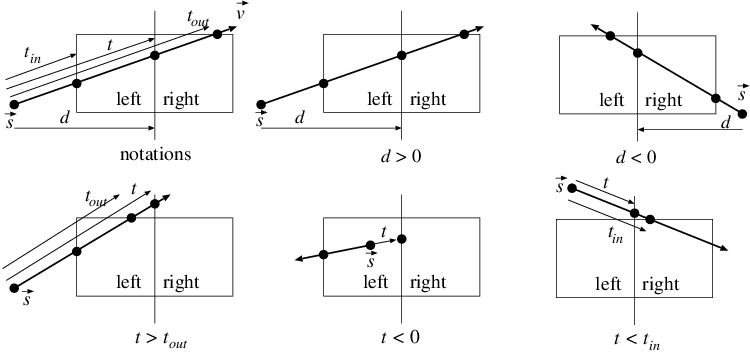
Similarly to the octree algorithm, the likelihood of successful intersections can be increased by continuing the tree building process until all empty spaces are cut (Figure 22.36).
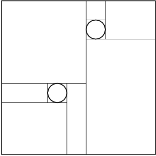
Our probabilistic world model contains spheres of same radius  , thus the non-empty cells are cubes of edge size
  . Unlike in uniform grids or octrees, the separating planes of kd-trees are not independent of the objects. Kd-tree splitting planes are rather tangents of the objects. This means that we do not have to be concerned with partially overlapping spheres since a sphere is completely contained by a cell in a kd-tree. The probability of the successful intersection is obtained applying Theorem 22.17. In the current case, the containing convex solid is a cube of edge size
  , the contained solid is a sphere of radius
  , thus the intersection probability is:
The expected number of intersection tests is then:
We can conclude that the kd-tree algorithm requires the smallest number of ray-surface intersection tests according to the probabilistic model.
Exercises
22.6-1 Prove that the expected number of intersection tests is constant in all those ray tracing algorithms which process objects in the order of their distance from the ray origin.
22.6-2 Propose a ray intersection algorithm for subdivision surfaces.
22.6-3 Develop a ray intersection method for B-spline surfaces.
22.6-4 Develop a ray intersection algorithm for CSG models assuming that the ray–primitive intersection tests are already available.
22.6-5 Propose a ray intersection algorithm for transformed objects assuming that the algorithm computing the intersection with the non-transformed objects is available (hints: transform the ray).
Rendering requires the identification of those surface points that are visible through the pixels of the virtual camera. Ray tracing solves this visibility problem for each pixel independently, thus it does not reuse visibility information gathered at other pixels. The algorithms of this section, however, exploit such information using the following simple techniques:
-
They simultaneously attack the visibility problem for all pixels, and handle larger parts of the scene at once.
-
Where feasible, they exploit the incremental principle which is based on the recognition that the visibility problem becomes simpler to solve if the solution at the neighbouring pixel is taken into account.
-
They solve each task in that coordinate system which makes the solution easier. The scene is transformed from one coordinate system to the other by homogeneous linear transformations.
-
They minimize unnecessary computations, therefore remove those objects by clipping in an early stage of rendering which cannot be projected onto the window of the camera.
Homogeneous linear transformations and clipping may change the type of the surface except for points, line segments and polygons.
Footnote. Although Bézier and B-Spline curves and surfaces are invariant to affine transformations, and NURBS is invariant even to homogeneous linear transformations, but clipping changes these object types as well.
Therefore, before rendering is started, each shape is approximated by points, line segments, and meshes (Subsection 22.3).
Figure 22.37. Steps of incremental rendering. (a) Modelling defines objects in their reference state. (b) Shapes are tessellated to prepare for further processing. (c) Modelling transformation places the object in the world coordinate system. (d) Camera transformation translates and rotates the scene to get the eye to be at the origin and to look parallel with axis . (e) Perspective transformation converts projection lines meeting at the origin to parallel lines, that is, it maps the eye position onto an ideal point. (f) Clipping removes those shapes and shape parts, which cannot be projected onto the window. (g) Hidden surface elimination removes those surface parts that are occluded by other shapes. (h) Finally, the visible polygons are projected and their projections are filled with their visible colours.
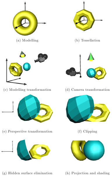
Steps of incremental rendering are shown in Figure 22.37. Objects are defined in their reference state, approximated by meshes, and are transformed to the virtual world. The time dependence of this transformation is responsible for object animation. The image is taken from the camera about the virtual world, which requires the identification of those surface points that are visible from the camera, and their projection onto the window plane. The visibility and projection problems could be solved in the virtual world as happens in ray tracing, but this would require the intersection calculations of general lines and polygons. Visibility and projection algorithms can be simplified if the scene is transformed to a coordinate system, where the  coordinates of a point equal to the coordinates of that pixel onto which this point is projected, and the
  coordinate can be used to decide which point is closer if more than one surfaces are projected onto the same pixel. Such coordinate system is called the screen coordinate system. In screen coordinates the units of axes
  and
and  are equal to the pixel size. Since it is usually not worth computing the image on higher accuracy than the pixel size, coordinates
  are integers. Because of performance reasons, coordinate
  is also often integer. Screen coordinates are denoted by capital letters.
The transformation taking to the screen coordinate system is defined by a sequence of transformations, and the elements of this sequence are discussed separately. However, this transformation is executed as a single multiplication with a  transformation matrix obtained as the product of elementary transformation matrices.
Rendering is expected to generate an image from a camera defined by eye position ( ) (the focal point of the camera), looking target (
 ) where the camera looks at, and by vertical direction
  (Figure 22.38).
Figure 22.38. Parameters of the virtual camera: eye position , target , and vertical direction , from which camera basis vectors are obtained, front and back clipping planes, and vertical field of view (the horizontal field of view is computed from aspect ratio ).
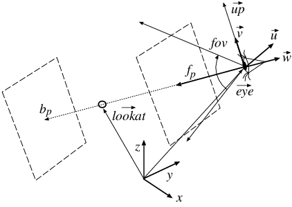
Camera parameter  defines the vertical field of view,
  is the ratio of the width and the height of the window,
  and
and  are the distances of the front and back clipping planes from the eye, respectively. These clipping planes allow to remove those objects that are behind, too close to, or too far from the eye.
We assign a coordinate system, i.e. three orthogonal unit basis vectors to the camera. Horizontal basis vector  , vertical basis vector
  , and basis vector
  pointing to the looking direction are obtained as follows:
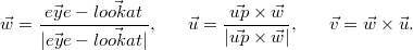
The camera transformation translates and rotates the space of the virtual world in order to get the camera to move to the origin, to look at direction axis  , and to have vertical direction parallel to axis
  , that is, this transformation maps unit vectors
  to the basis vectors of the coordinate system. Transformation matrix
  can be expressed as the product of a matrix translating the eye to the origin and a matrix rotating basis vectors
  of the camera to the basis vectors of the coordinate system:
where
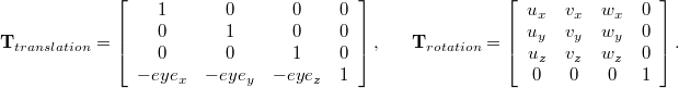
Let us note that the columns of the rotation matrix are vectors  . Since these vectors are orthogonal, it is easy to see that this rotation maps them to coordinate axes
  . For example, the rotation of vector
  is:
is:

In the next step the viewing pyramid containing those points which can be projected onto the window is normalized making the field of view equal to 90 degrees (Figure 22.39).
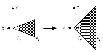
Normalization is a simple scaling transformation:
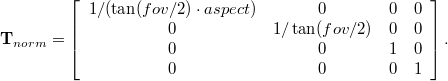
The main reason of this transformation is to simplify the formulae of the next transformation step, called perspective transformation.
The perspective transformation distorts the virtual world to allow the replacement of the perspective projection by parallel projection during rendering.
After the normalizing transformation, the potentially visible points are inside a symmetrical finite frustum of pyramid of 90 degree apex angle (Figure 22.39). The perspective transformation maps this frustum onto a cube, converting projection lines crossing the origin to lines parallel to axis  (Figure 22.40).
Figure 22.40. The perspective transformation maps the finite frustum of pyramid defined by the front and back clipping planes, and the edges of the window onto an axis aligned, origin centred cube of edge size 2.
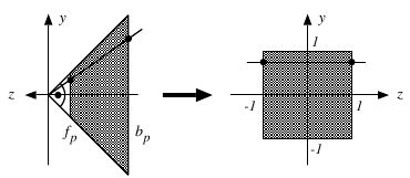
Perspective transformation is expected to map point to point, line to line, but to map the eye position to infinity. It means that perspective transformation cannot be a linear transformation of Cartesian coordinates. Fortunately, homogeneous linear transforms also map point to point, line to line, and are able to handle points at infinity with finite coordinates. Let us thus try to find the perspective transformation in the form of a homogeneous linear transformation defined by a  matrix:
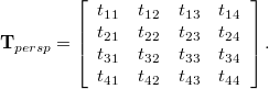
Figure 22.40 shows a line (projection ray) and its transform. Let  and
and  be the
  and the
  slopes of the line, respectively. This line is defined by equation
 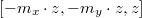 in the normalized camera space. The perspective transformation maps this line to a “horizontal” line crossing point
  and being parallel to axis
  . Let us examine the intersection points of this line with the front and back clipping planes, that is, let us substitute
  and
and  into parameter
  of the line equation. The transformation should map these points to
  and
and  , respectively.
The perspective transformation of the point on the first clipping plane is:

where  is an arbitrary, non-zero scalar since the point defined by homogeneous coordinates does not change if the homogeneous coordinates are simultaneously multiplied by a non-zero scalar. Setting
  to
to  , we get:

Note that the first coordinate of the transformed point equals to the first coordinate of the original point on the clipping plane for arbitrary  ,
,  , and
, and  values. This is possible only if the first column of matrix
  is
is  . Using the same argument for the second coordinate, we can conclude that the second column of the matrix is
  . Furthermore, in equation (22.32) the third and the fourth homogeneous coordinates of the transformed point are not affected by the first and the second coordinates of the original point, requiring
  . The conditions on the third and the fourth homogeneous coordinates can be formalized by the following equations:

Applying the same procedure for the intersection point of the projection line and the back clipping plane, we can obtain other two equations:

Solving this system of linear equations, the matrix of the perspective transformation can be expressed as:
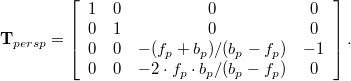
Since perspective transformation is not affine, the fourth homogeneous coordinate of the transformed point is usually not 1. If we wish to express the coordinates of the transformed point in Cartesian coordinates, the first three homogeneous coordinates should be divided by the fourth coordinate. Homogeneous linear transforms map line segment to line segment and triangle to triangle, but it may happen that the resulting line segment or triangle contains ideal points (Subsection 22.5.2). The intuition behind the homogeneous division is a traveling from the projective space to the Euclidean space, which converts a line segment containing an ideal point to two half lines. If just the two endpoints of the line segment is transformed, then it is not unambiguous whether the two transformed points need to be connected by a line segment or the complement of this line segment should be considered as the result of the transformation. This ambiguity is called the wrap around problem.
The wrap around problem does not occur if we can somehow make sure that the original shape does not contain points that might be mapped onto ideal points. Examining the matrix of the perspective transformation we can conclude that the fourth homogeneous coordinate of the transformed point will be equal to the  coordinate of the original point. Ideal points having zero fourth homogeneous coordinate (
 ) may thus be obtained transforming the points of plane
  , i.e. the plane crossing the origin and parallel to the window. However, if the shapes are clipped onto a first clipping plane being in front of the eye, then these points are removed. Thus the solution of the wrap around problem is the execution of the clipping step before the homogeneous division.
The purpose of clipping is to remove all shapes that either cannot be projected onto the window or are not between the front and back clipping planes. To solve the wrap around problem, clipping should be executed before the homogeneous division. The clipping boundaries in homogeneous coordinates can be obtained by transforming the screen coordinate AABB back to homogeneous coordinates. In screen coordinates, i.e. after homogeneous division, the points to be preserved by clipping meet the following inequalities:

On the other hand, points that are in front of the eye after camera transformation have negative  coordinates, and the perspective transformation makes the fourth homogeneous coordinate
  equal to
  in normalized camera space. Thus the fourth homogeneous coordinate of points in front of the eye is always positive. Let us thus add condition
  to the set of conditions of inequalities (22.33). If
  is positive, then inequalities (22.33) can be multiplied by
  , resulting in the definition of the clipping region in homogeneous coordinates:

Points can be clipped easily, since we should only test whether or not the conditions of inequalities (22.34) are met. Clipping line segments and polygons, on the other hand, requires the computation of the intersection points with the faces of the clipping boundary, and only those parts should be preserved which meet inequalities (22.34).
Clipping algorithms using Cartesian coordinates were discussed in Subsection 22.4.3. Those methods can also be applied in homogeneous coordinates with two exceptions. Firstly, for homogeneous coordinates, inequalities (22.34) define whether a point is in or out. Secondly, intersections should be computed using the homogeneous coordinate equations of the line segments and the planes.
Let us consider a line segment with endpoints  and
and  . This line segment can be an independent shape or an edge of a polygon. Here we discuss the clipping on half space of equation
  (clipping methods on other half spaces are very similar). Three cases need to be distinquished:
-
If both endpoints of the line segment are inside, that is
 and
and  , then the complete line segment is in, thus is preserved.
 -
If both endpoints are outside, that is
 and
and  , then all points of the line segment are out, thus it is completely eliminated by clipping.
 -
If one endpoint is outside, while the other is in, then the intersection of the line segment and the clipping plane should be obtained. Then the endpoint being out is replaced by the intersection point. Since the points of a line segment satisfy equation (22.18), while the points of the clipping plane satisfy equation
 , parameter
  of the intersection point is computed as:
 Substituting parameter
 into the equation of the line segment, homogeneous coordinates
  of the intersection point are obtained.

Clipping may introduce new vertices. When the vertices have some additional features, for example, the surface colour or normal vector at these vertices, then these additional features should be calculated for the new vertices as well. We can use linear interpolation. If the values of a feature at the two endpoints are  and
and  , then the feature value at new vertex
  generated by clipping is
  .
.
Having executed the perspective transformation, the Cartesian coordinates of the visible points are in  . These normalized device coordinates should be further scaled and translated according to the resolution of the screen and the position of the viewport where the image is expected. Denoting the left-bottom corner pixel of the screen viewport by
  , the right-top corner by
  , and
, and  coordinates expressing the distance from the eye are expected in
  , the matrix of the viewport transformation is:
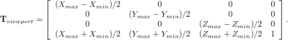
Coordinate systems after the perspective transformation are left handed, unlike the coordinate systems of the virtual world and the camera, which are right handed. Left handed coordinate systems seem to be unusual, but they meet our natural expectation that the screen coordinate  grows from left to right, the
  coordinate from bottom to top and, the
  coordinate grows in the direction of the camera target.
After clipping, homogeneous division, and viewport transformation, shapes are in the screen coordinate system where a point of coordinates  can be assigned to a pixel by extracting the first two Cartesian coordinates
  .
.
Rasterization works in the screen coordinate system and identifies those pixels which have to be coloured to approximate the projected shape. Since even simple shapes can cover many pixels, rasterization algorithms should be very fast, and should be appropriate for hardware implementation.
Let the endpoints of a line segment be  and
and  in screen coordinates. Let us further assume that while we are going from the first endpoint towards the second, both coordinates are growing, and
  is the faster changing coordinate, that is,

In this case the line segment is moderately ascending. We discuss only this case, other cases can be handled by exchanging the  coordinates and replacing additions by substractions.
Line drawing algorithms are expected to find pixels that approximate a line in a way that there are no holes and the approximation is not fatter than necessary. In case of moderately ascending line segments this means that in each pixel column exactly one pixel should be filled with the colour of the line. This coloured pixel is the one closest to the line in this column. Using the following equation of the line

in pixel column of coordinate  , the pixel closest to the line has
  coordinate that is equal to the rounding of
  . Unfortunately, the determination of
  requires a floating point multiplication, addition, and a rounding operation, which are too slow.
In order to speed up line drawing, we apply a fundamental trick of computer graphics, the incremental principle. The incremental principle is based on the recognition that it is usually simpler to evaluate a function  using value
  than computing it from
  . Since during line drawing the columns are visited one by one, when column
  is processed, value
  is already available. In case of a line segment we can write:

Note that the evaluation of this formula requires just a single floating point addition ( is less than 1). This fact is exploited in digital differential analyzator algorithms (DDA-algorithms). The DDA line drawing algorithm is then:
DDA-Line-Drawing(
)
12
3
FOR
TO4
DORound()5Pixel-Write()6


Further speedups can be obtained using fixed point number representation. This means that the product of the number and  is stored in an integer variable, where
  is the number of fractional bits. The number of fractional bits should be set to exclude cases when the rounding errors accumulate to an incorrect result during long iteration sequences. If the longest line segment covers
  columns, then the minimum number of fractional bits guaranteeing that the accumulated error is less than 1 is
  . Thanks to clipping only lines fitting to the screen are rasterized, thus
  is equal to the maximum screen resolution.
The performance and simplicity of the DDA line drawing algorithm can still be improved. On the one hand, the software implementation of the DDA algorithm requires shift operations to realize truncation and rounding operations. On the other hand – once for every line segment – the computation of slope  involves a division which is computationally expensive. Both problems are solved in the Bresenham line drawing algorithm.
Figure 22.41. Notations of the Bresenham algorithm: is the signed distance between the closest pixel centre and the line segment along axis , which is positive if the line segment is above the pixel centre. is the distance along axis between the pixel centre just above the closest pixel and the line segment.
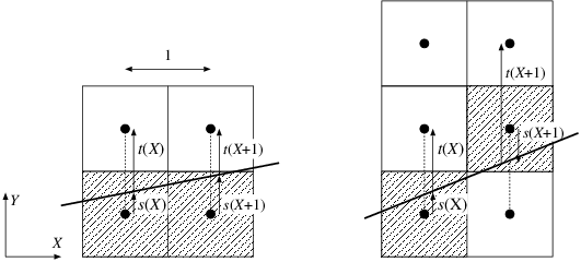
Let us denote the vertical, signed distance of the line segment and the closest pixel centre by  , and the vertical distance of the line segment and the pixel centre just above the closest pixel by
  (Figure 22.41). As the algorithm steps onto the next pixel column, values
  and
and  change and should be recomputed. While the new
  and
and  values satisfy inequality
  , that is, while the lower pixel is still closer to the line segment, the shaded pixel of the next column is in the same row as in the previous column. Introducing error variable
  , the row of the shaded pixel remains the same until this error variable is negative (
 ). As the pixel column is incremented, variables
  are updated using the incremental formulae (
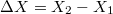 ,
, 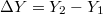 ):
):

These formulae are valid if the closest pixel in column  is in the same row as in column
  . If stepping to the next column, the upper pixel gets closer to the line segment (error variable
  becomes positive), then variables
  should be recomputed for the new closest row and for the pixel just above it. The formulae describing this case are as follows:

Note that  is a signed distance which is negative if the line segment is below the closest pixel centre, and positive otherwise. We can assume that the line starts at a pixel centre, thus the initial values of the control variables are:

This algorithm keeps updating error variable  and steps onto the next pixel row when the error variable becomes positive. In this case, the error variable is decreased to have a negative value again. The update of the error variable requires a non-integer addition and the computation of its increment involves a division, similarly to the DDA algorithm. It seems that this approach is not better than the DDA.
Let us note, however, that the sign changes of the error variable can also be recognized if we examine the product of the error variable and a positive number. Multiplying the error variable by  we obtain decision variable
  . In case of moderately ascending lines the decision and error variables change their sign simultaneously. The incremental update formulae of the decision variable can be obtained by multiplying the update formulae of error variable by
  :
:
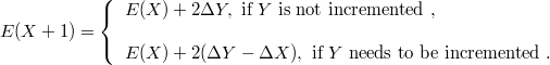
The initial value of the decision variable is  .
.
The decision variable starts at an integer value and is incremented by integers in each step, thus it remains to be an integer and does not require fractional numbers at all. The computation of the increments need only integer additions or subtractions and multiplications by 2.
The complete Bresenham line drawing algorithm is:
Bresenham-Line-Drawing(
)
12
3
4
5
6
FOR
TO7
DOIF8
THEN
The line stays in the current pixel row. 9
ELSE
The line steps onto the next pixel row. 10
11
Pixel-Write()

The fundamental idea of the Bresenham algorithm was the replacement of the fractional error variable by an integer decision variable in a way that the conditions used by the algorithm remained equivalent. This approach is also called the method of invariants, which is useful in many rasterization algorithms.
The input of an algorithm filling single connected polygons is the array of vertices  (this array is usually the output of the polygon clipping algorithm). Edge
  of the polygon connects vertices
  and
and  . The last vertex needs not be treated in a special way if the first vertex is put again after the last vertex in the array. Multiply connected polygons are defined by more than one closed polylines, thus are specified by more than one vertex arrays.
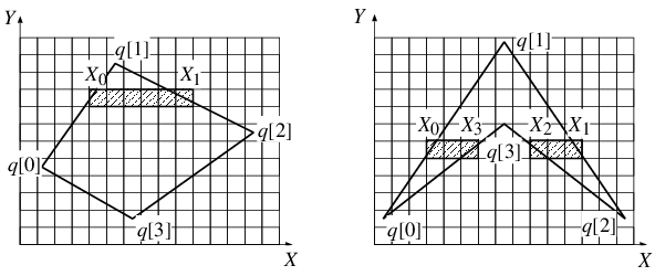
The filling is executed by processing a horizontal pixel row called scan line at a time. For a single scan line, the pixels belonging to the interior of the polygon can be found by the following steps. First the intersections of the polygon edges and the scan line are calculated. Then the intersection points are sorted in the ascending order of their  coordinates. Finally, pixels between the first and the second intersection points, and between the third and the fourth intersection points, or generally between the
  th and the
  th intersection points are set to the colour of the polygon (Figure 22.42). This algorithm fills those pixels which can be reached from infinity by crossing the polygon boundary odd number of times.
The computation of the intersections between scan lines and polygon edges can be speeded up using the following observations:
-
An edge and a scan line can have intersection only if coordinate
 of the scan line is between the minimum and maximum
  coordinates of the edge. Such edges are the active edges. When implementing this idea, an active edge table (AET for short) is needed which stores the currently active edges.
 -
The computation of the intersection point of a line segment and the scan line requires floating point multiplication, division, and addition, thus it is time consuming. Applying the incremental principle, however, we can also obtain the intersection point of the edge and a scan line from the intersection point with the previous scan line using a single, fixed-point addition (Figure 22.43).
Figure 22.43. Incremental computation of the intersections between the scan lines and the edges. Coordinate always increases with the reciprocal of the slope of the line.
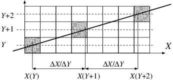
When the incremental principle is exploited, we realize that coordinate  of the intersection with an edge always increases by the same amount when scan line
  is incremented. If the edge endpoint having the larger
  coordinate is
  and the endpoint having the smaller
  coordinate is
  , then the increment of the
  coordinate of the intersection is
  , where
  and
and  . This increment is usually not an integer, hence increment
  and intersection coordinate
  should be stored in non-integer, preferably fixed-point variables. An active edge is thus represented by a fixed-point increment
  , the fixed-point coordinate value of intersection
  , and the maximum vertical coordinate of the edge (
 ). The maximum vertical coordinate is needed to recognize when the edge becomes inactive.

Scan lines are processed one after the other. First, the algorithm determines which edges become active for this scan line, that is, which edges have minimum  coordinate being equal to the scan line coordinate. These edges are inserted into the active edge table. The active edge table is also traversed and those edges whose maximum
  coordinate equals to the scan line coordinate are removed (note that this way the lower end of an edge is supposed to belong to the edge, but the upper edge is not). Then the active edge table is sorted according to the
  coordinates of the edges, and the pixels between each pair of edges are filled. Finally, the
  coordinates of the intersections in the edges of the active edge table are prepared for the next scan line by incrementing them by the reciprocal of the slope
  .
.
Polygon-Fill(
)
1FORTO2
DOFOReachof

Put activated edges into the AET. 3
DOIF4
THENPut-AET()5FOReachof the AET
Remove deactivated edges from the AET. 6
DOIF7
THENDelete-from-AET()8Sort-AETSort according to
. 9
FOReach pair of edgesof the AET 10
DOFORRound()TORound()11DOPixel-Write()12FOReachin the AET
Incremental principle. 13
DO


The algorithm works scan line by scan line and first puts the activated edges  to the active edge table. The active edge table is maintained by three operations. Operation
 Put-AET(
) computes variables  of an edge and inserts this structure into the table. Operation
 Delete-from-AET removes an item from the table when the edge is not active any more  . Operation
 Sort-AET sorts the table in the ascending order of the  value of the items. Having sorted the lists, every two consecutive items form a pair, and the pixels between the endpoints of each of these pairs are filled. Finally, the
  coordinates of the items are updated according to the incremental principle.
The three-dimensional visibility problem is solved in the screen coordinate system. We can assume that the surfaces are given as triangle meshes.
The z-buffer algorithm finds that surface for each pixel, where the  coordinate of the visible point is minimal. For each pixel we allocate a memory to store the minimum
  coordinate of those surfaces which have been processed so far. This memory is called the z-buffer or the depth-buffer.
When a triangle of the surface is rendered, all those pixels are identified which fall into the interior of the projection of the triangle by a triangle filling algorithm. As the filling algorithm processes a pixel, the  coordinate of the triangle point visible in this pixel is obtained. If this
  value is larger than the value already stored in the z-buffer, then there exists an already processed triangle that is closer than the current triangle in this given pixel. Thus the current triangle is obscured in this pixel and its colour should not be written into the raster memory. However, if the new
  value is smaller than the value stored in the z-buffer, then the current triangle is the closest so far, and its colour and
  coordinate should be written into the pixel and the z-buffer, respectively.
The z-buffer algorithm is then:
Z-buffer()
1FOReach pixel
Clear screen. 2
DOPixel-Write()3maximum value after clipping 4
FOReach triangle
Rendering. 5
DOFOReach pixelof triangle
6
DOcoordinate
of that point
which projects onto pixel
7
IF8
THENPixel-Write(, colour of trianglein this point)9


When the triangle is filled, the general polygon filling algorithm of the previous section could be used. However, it is worth exploiting the special features of the triangle. Let us sort the triangle vertices according to their  coordinates and assign index 1 to the vertex of the smallest
  coordinate and index 3 to the vertex of the largest
  coordinate. The third vertex gets index 2. Then let us cut the triangle into two pieces with scan line
  . After cutting we obtain a “lower” triangle and an “upper” triangle. Let us realize that in such triangles the first (left) and the second (right) intersections of the scan lines are always on the same edges, thus the administration of the polygon filling algorithm can be significantly simplified. In fact, the active edge table management is not needed anymore, only the incremental intersection calculation should be implemented. The classification of left and right intersections depend on whether
  is on the right or on the left side of the oriented line segment from
  to
to  . If
. If  is on the left side, the projected triangle is called left oriented, and right oriented otherwise.
When the details of the algorithm is introduced, we assume that the already re-indexed triangle vertices are

The rasterization algorithm is expected to fill the projection of this triangle and also to compute the  coordinate of the triangle in every pixel (Figure 22.45).
Figure 22.45. A triangle in the screen coordinate system. Pixels inside the projection of the triangle on plane need to be found. The coordinates of the triangle in these pixels are computed using the equation of the plane of the triangle.
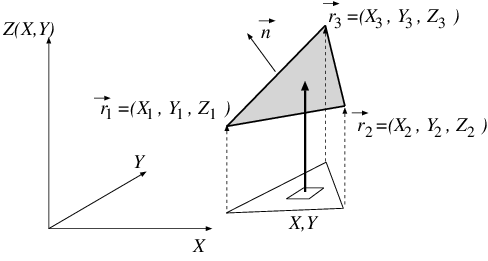
The  coordinate of the triangle point visible in pixel
  is computed using the equation of the plane of the triangle (equation (22.1)):

where 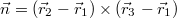 and
and  . Whether the triangle is left oriented or right oriented depends on the sign of the
  coordinate of the normal vector of the plane. If
  is negative, then the triangle is left oriented. If it is negative, then the triangle is right oriented. Finally, when
  is zero, then the projection maps the triangle onto a line segment, which can be ignored during filling.
Using the equation of the plane, function  expressing the
  coordinate corresponding to pixel
  is:
is:

According to the incremental principle, the evaluation the  coordinate can take advantage of the value of the previous pixel:

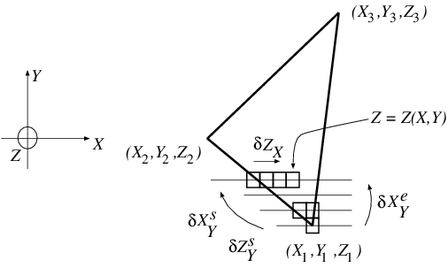
Since increment  is constant for the whole triangle, it needs to be computed only once. Thus the calculation of the
  coordinate in a scan line requires just a single addition per pixel. The
  coordinate values along the edges can also be obtained incrementally from the respective values at the previous scan line (Figure 22.46). The complete incremental algorithm which renders a lower left oriented triangle is as follows (the other cases are very similar):
Z-buffer-Lower-Triangle(
)
1
Normal vector. 2

increment. 3
4
5
FOR
TO6
DO7
FORRound()TORound()One scan line. 8
DOIF
Visibility test. 9
THENPixel-Write()1011
12

Next scan line.


This algorithm simultaneously identifies the pixels to be filled and computes the  coordinates with linear interpolation. Linear interpolation requires just a single addition when a pixel is processed. This idea can also be used for other features as well. For example, if the colour of the triangle vertices are available, the colour of the internal points can be set to provide smooth transitions applying linear interpolation. Note also that the addition to compute the feature value can also be implemented by a special purpose hardware. Graphics cards have a great number of such interpolation units.
If a pixel of the image corresponds to a given object, then its neighbours usually correspond to the same object, that is, visible parts of objects appear as connected territories on the screen. This is a consequence of object coherence and is called image coherence.
Figure 22.47. Polygon-window relations:: (a) distinct; (b) surrounding ; (c) intersecting; (d) contained.
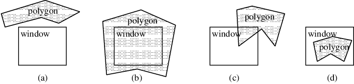
If the situation is so fortunate—from a labor saving point of view—that a polygon in the object scene obscures all the others and its projection onto the image plane covers the image window completely, then we have to do no more than simply fill the image with the colour of the polygon. If no polygon edge falls into the window, then either there is no visible polygon, or some polygon covers it completely (Figure 22.47). The window is filled with the background colour in the first case, and with the colour of the closest polygon in the second case. If at least one polygon edge falls into the window, then the solution is not so simple. In this case, using a divide-and-conquer approach, the window is subdivided into four quarters, and each subwindow is searched recursively for a simple solution.
The basic form of the algorithm called Warnock-algorithm rendering a rectangular window with screen coordinates  (lower left corner) and
  (upper right corner) is this:
Warnock(
)
1IFor

Is the window larger than a pixel? 2
THENIFat least one edge projects onto the window 3THENNon-trivial case: Subdivision and recursion. 4
Warnock()5Warnock()6Warnock()7Warnock()8ELSETrivial case: window
is homogeneous. 9
the polygon visible in pixel
10
IFno visible polygon 11THENfill rectanglewith the background colour 12 tab/>
ELSEfill rectanglewith the colour of


Note that the algorithm can handle non-intersecting polygons only. The algorithm can be accelerated by filtering out those distinct polygons which can definitely not be seen in a given subwindow at a given step. Furthermore, if a surrounding polygon appears at a given stage, then all the others behind it can be discarded, that is all those which fall onto the opposite side of it from the eye. Finally, if there is only one contained or intersecting polygon, then the window does not have to be subdivided further, but the polygon (or rather the clipped part of it) is simply drawn. The price of saving further recurrence is the use of a scan-conversion algorithm to fill the polygon.
If we simply scan convert polygons into pixels and draw the pixels onto the screen without any examination of distances from the eye, then each pixel will contain the colour of the last polygon falling onto that pixel. If the polygons were ordered by their distance from the eye, and we took the farthest one first and the closest one last, then the final picture would be correct. Closer polygons would obscure farther ones — just as if they were painted an opaque colour. This method is known as the painter's algorithm.
The only problem is that the order of the polygons necessary for performing the painter's algorithm is not always simple to compute. We say that a polygon  does not obscure another polygon
  if none of the points of
  is obscured by
  . To have this relation, one of the following conditions should hold
-
Polygons
 and
and  do not overlap in
  range, and the minimum
  coordinate of polygon
  is greater than the maximum
  coordinate of polygon
  .
. -
The bounding rectangle of
 on the
  plane does not overlap with that of
  .
. -
Each vertex of
 is farther from the viewpoint than the plane containing
  .
. -
Each vertex of
 is closer to the viewpoint than the plane containing
  .
. -
The projections of
 and
and  do not overlap on the
  plane.
All these conditions are sufficient. The difficulty of their test increases, thus it is worth testing the conditions in the above order until one of them proves to be true. The first step is the calculation of an initial depth order. This is done by sorting the polygons according to their maximal  value into a list. Let us first take the polygon
  which is the last item on the resulting list. If the
  range of
  does not overlap with any of the preceding polygons, then
  is correctly positioned, and the polygon preceding
  can be taken instead of
  for a similar examination. Otherwise
  overlaps a set
  of polygons. The next step is to try to check whether
  does not obscure any of the polygons in
  , that is, that
  is at its right position despite the overlapping. If it turns out that
  obscures
  for a polygon in the set
  , then
  has to be moved behind
  in the list, and the algorithm continues stepping back to
  . Unfortunately, this algorithm can run into an infinite loop in case of cyclic overlapping. Cycles can be resolved by cutting. In order to accomplish this, whenever a polygon is moved to another position in the list, we mark it. If a marked polygon
  is about to be moved again, then — assuming that
  is a part of a cycle —
  is cut into two pieces
  by the plane of
  , so that
  does not obscure
  and
and  does not obscure
  , and only
  is moved behind
  .
.
Binary space partitioning divides first the space into two halfspaces, the second plane divides the first halfspace, the third plane divides the second halfspace, further planes split the resulting volumes, etc. The subdivision can well be represented by a binary tree, the so-called BSP-tree illustrated in Figure 22.48. The kd-tree discussed in Subsection 22.6.2 is also a special version of BSP-trees where the splitting planes are parallel with the coordinate planes. The BSP-tree of this subsection, however, uses general planes.
The first splitting plane is associated with the root node of the BSP-tree, the second and third planes are associated with the two children of the root, etc. For our application, not so much the planes, but rather the polygons defining them, will be assigned to the nodes of the tree, and the set of polygons contained by the volume is also necessarily associated with each node. Each leaf node will then contain either no polygon or one polygon in the associated set.
The BSP-Tree-Construction algorithm for creating the BSP-tree for a set  of polygons uses the following notations. A node of the binary tree is denoted by
  , the polygon associated with the node by
  , and the two child nodes by
  and
and  , respectively. Let us consider a splitting plane of normal
  and place vector
  . Point
  belongs to the positive (right) subspace of this plane if the sign of scalar product
  is positive, otherwise it is in the negative (left) subspace. The BSP construction algorithm is:
BSP-Tree-Construction(
)
1 Create a new2
IFis empty or contains just a single polygon 3
THEN4
5
6
ELSEone polygon from list
7 Remove polygon
from list
8
polygons of
which overlap with the positive subspace of
9
polygons of
which overlap with the negative subspace of
10
BSP-Tree-Construction()11BSP-Tree-Construction()12RETURN


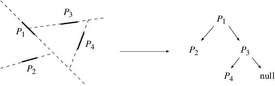
The size of the BSP-tree, i.e. the number of polygons stored in it, is on the one hand highly dependent on the nature of the object scene, and on the other hand on the “choice strategy” used when one polygon from list  is selected.
Having constructed the BSP-tree the visibility problem can be solved by traversing the tree in the order that if a polygon obscures another than it is processed later. During such a traversal, we determine whether the eye is at the left or right subspace at each node, and continue the traversal in the child not containing the eye. Having processed the child not containing the eye, the polygon of the node is drawn and finally the child containing the eye is traversed recursively.
Exercises
22.7-1 Implement the complete Bresenham algorithm that can handle not only moderately ascending but arbitrary line segments.
22.7-2 The presented polygon filling algorithm tests each edges at a scan line whether it becomes active here. Modify the algorithm in a way that such tests are not executed at each scan line, but only once.
22.7-3 Implement the complete z-buffer algorithm that renders left/righ oriented, upper/lower triangles.
22.7-4 Improve the presented Warnock-algorithm and eliminate further recursions when only one edge is projected onto the subwindow.
22.7-5 Apply the BSP-tree for discrete time collision detection.
22.7-6 Apply the BSP-tree as a space partitioning structure for ray tracing.
PROBLEMS |
22-1 Ray tracing renderer
Implement a rendering system applying the ray tracing algorithm. Objects are defined by triangle meshes and quadratic surfaces, and are associated with diffuse reflectivities. The virtual world also contains point light sources. The visible colour of a point is proportional to the diffuse reflectivity, the intensity of the light source, the cosine of the angle between the surface normal and the illumination direction (Lambert's law), and inversely proportional with the distance of the point and the light source. To detect whether or not a light source is not occluded from a point, use the ray tracing algorithm as well.
22-2 Continuous time collision detection with ray tracing
Using ray tracing develop a continuous time collision detection algorithm which computes the time of collision between a moving and rotating polyhedron and a still half space. Approximate the motion of a polygon vertex by a uniform, constant velocity motion in small intervals  .
.
22-3 Incremental rendering system
Implement a three-dimensional renderer based on incremental rendering. The modelling and camera transforms can be set by the user. The objects are given as triangle meshes, where each vertex has colour information as well. Having transformed and clipped the objects, the z-buffer algorithm should be used for hidden surface removal. The colour at the internal points is obtained by linear interpolation from the vertex colours.
CHAPTER NOTES |
The elements of Euclidean, analytic and projective geometry are discussed in the books of Maxwell [238], [237] and Coxeter [76]. The application of projective geometry in computer graphics is presented in Herman's dissertation [163] and Krammer's paper [205]. Curve and surface modelling is the main focus of computer aided geometric design (CAD, CAGD), which is discussed by Gerald Farin [103], and Rogers and Adams [289]. Geometric models can also be obtained measuring real objects, as proposed by reverse engineering methods [335]. Implicit surfaces can be studied by reading Bloomenthal's work [45]. Solid modelling with implicit equations is also booming thanks to the emergence of functional representation methods (F-Rep), which are surveyed at http://cis.k.hosei.ac.jp/~F-rep. Blobs have been first proposed by Blinn [44]. Later the exponential influence function has been replaced by polynomials [347], which are more appropriate when roots have to be found in ray tracing.
Geometric algorithms give solutions to geometric problems such as the creation of convex hulls, clipping, containment test, tessellation, point location, etc. This field is discussed in the books of Preparata and Shamos [278] and of Marc de Berg [81], [82]. The triangulation of general polygons is still a difficult topic despite to a lot of research efforts. Practical triangulation algorithms run in  [82], [298], [355], but Chazelle [62] proposed an optimal algorithm having linear time complexity. The presented proof of the two ears theorem has originally been given by Joseph O'Rourke [260]. Subdivision surfaces have been proposed and discussed by Catmull and Clark [59], Warren and Weimer [338], and by Brian Sharp [301], [300]. The butterfly subdivision approach has been published by Dyn et al. [95]. The Sutherland–Hodgeman polygon clipping algorithm is taken from [309].
Collision detection is one of the most critical problems in computer games since it prevents objects to fly through walls and it is used to decide whether a bullet hits an enemy or not. Collision detection algorithms are reviewed by Jiménez, Thomas and Torras [183].
Glassner's book [133] presents many aspects of ray tracing algorithms. The 3D DDA algorithm has been proposed by Fujimoto et al. [122]. Many papers examined the complexity of ray tracing algorithms. It has been proven that for  objects, ray tracing can be solved in
  time [81], [312], but this is theoretical rather than practical result since it requires
  memory and preprocessing time, which is practically unacceptable. In practice, the discussed heuristic schemes are preferred, which are better than the naive approach only in the average case. Heuristic methods have been analyzed by probabilistic tools by Márton [312], who also proposed the probabilistic scene model used in this chapter as well. We can read about heuristic algorithms, especially about the efficient implementation of the kd-tree based ray tracing in Havran's dissertation [158]. A particularly efficient solution is given in Szécsi's paper [310].
The probabilistic tools, such as the Poisson point process can be found in the books of Karlin and Taylor [189] and Lamperti [211]. The cited fundamental law of integral geometry can be found in the book of Santaló [295].
The geoinformatics application of quadtrees and octrees are also discussed in chapter 16 of this book.
The algorithms of incremental image synthesis are discussed in many computer graphics textbooks [114]. Visibility algorithms have been compared in [309], [311]. The painter's algorithm has been proposed by Newell et al. [255]. Fuchs examined the construction of minimal depth BSP-trees [121]. The source of the Bresenham algorithm is [48].
Graphics cards implement the algorithms of incremental image synthesis, including transformations, clipping, z-buffer algorithm, which are accessible through graphics libraries (OpenGL, DirectX). Current graphics hardware includes two programmable processors, which enables the user to modify the basic rendering pipeline. Furthermore, this flexibility allows non graphics problems to be solved on the graphics hardware. The reason of using the graphics hardware for non graphics problems is that graphics cards have much higher computational power than CPUs. We can read about such algorithms in the ShaderX or in the GPU Gems [106] series or visiting the http://www.gpgpu.org web page.
Table of Contents
In the internet—within http://www.hcibib.org/—the following definition is found: “Human-computer interaction is a discipline concerned with the design, evaluation and implementation of interactive computing systems for human use and with the study of major phenomena surrounding them ... . Some of its special concerns are:
-
the joint performance of tasks by humans and machines;
-
the structure of communication between human and machine;
-
human capabilities to use machines (including the learnability of interfaces);
-
algorithms and programming of the interface itself;
-
engineering concerns that arise in designing and building interfaces;
-
the process of specification, design, and implementation of interfaces.
... Human-computer interaction thus has science, engineering, and design aspects.”
Many of these topics do only marginally concern algorithms in the classical sense. Therefore, in this chapter we concentrate on human-computer scenario for problem solving where the machines are forced to do lots of computation, and the humans have a role as intelligent controllers and directors.
Humans are able to think, to feel, and to sense—and they adopt quickly to a new situation. We can also compute, but not too well. In contrast, computers are giants in computing—they crunch bits and bytes like maniacs. However, they cannot do anything else but computing—especially they are not very flexible. Combining the different gifts and strengths of humans and machines in appropriate ways may lead to impressive performances.
One suitable approach for such team work is “Multiple-Choice Optimisation”. In a “Multiple-Choice System” the computer gives a clear handful of candidate solutions, two or three or five ... Then a human expert makes the final choice amongst these alternatives. One key advantage of a proper multiple-choice approach is that the human is not drown by deluges of data.
Multiple-Choice Systems may be especially helpful in realtime scenarios of the following type: In principle there is enough time to compute a perfect solution. But certain parameters of the problem are unknown or fuzzy. They concretise only in a very late moment, when there is no more time for elaborate computations. Now assume that the decision maker has used multiple-choice algorithms to generate some good candidate solutions in beforehand. When the exact problem data show up he may select an appropriate one of these alternatives in realtime.
An example from vehicle routing is given. A truck driver has to go from A to Z. Before the trip he uses PC software to find two or three different good routes and prints them out. During the trip radio gives information on current traffic jams or weather problems. In such moments the printed alternatives help the driver to switch routes in realtime.
However, it is not at all easy to have the computer finding good small samples of solutions. Naively, the most natural way seems to be the application of  -best algorithms: Given a (discrete) optimisation problem with some objective function, the
  best solutions are computed for a prescribed integer
  . However, such
  -best solutions tend to be micro mutations of each other instead of true alternatives.
Figure 23.1 exhibits a typical pattern: In a grid graph of dimension  the goal was to find short paths from the lower left to the upper right corner. The edge lengths are random numbers, not indicated in the diagram. The 1000 (!) shortest paths were computed, and their union is shown in the figure. The similarity amongst all these paths is striking. Watching the picture from a somewhat larger distance will even give the impression of only a single path, drawn with a bushy pencil. (The computation of alternative short paths will also be the most prominent example case in Section 23.2)
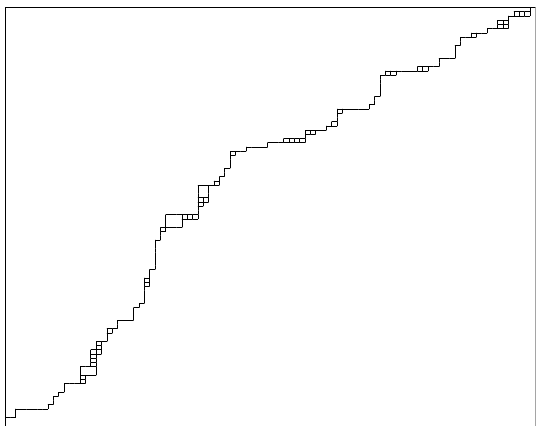
Often the term “multiple-choice” is used in the context of “multiple-choice tests”. This means something completely different. The difference between multiple-choice optimisation and multiple-choice tests lies in the type and quality of the candidate solutions:
-
In multiple-choice tests always at least one of the answers is “correct”, whereas others may be right or wrong. Beforehand an authority (the test designer) has prepared the question together with the candidate answers and the decision which of them are correct ones.
-
In the optimisation situation nothing is clear: Perhaps all of the candidate solutions are ok, but it may also be that they all are not appropriate. And there is typically no master who tells the human whether his choice is good or not. Because of this uncertainty many humans really need some initiation time to accept their role within a multiple-choice system.
(1) Short Paths
Starting in the early 1990's, PC programs for vehicle routing have become more and more popular. In 1997 the Dutch software company AND was first to sell such a program which did not only compute the “best” (= shortest or quickest) route but also one or two alternatives. The user had the choice to request all these candidate solutions simultaneously or one after the other. The user was also allowed to determine some parameters for route visualisation, namely different colours and thickness for best, second, third choice. Related is work by F. Berger. She developed a method to identify linear structures (like roads, rails, rivers, ...) in grey level satellite images. Typically, candidate structures are not unique, and the algorithm of Berger makes several alternative proposals. The Berger method is based on algorithms for generating short alternative paths.
(2) Travelling Salesperson Problem and the Drilling of Holes in Circuit Boards
In the Travelling Salesperson Problem (TSP)  locations are given and their mutual distances. The task is to find a shortest round trip through all
  points. TSP is NP-complete. One important application in electronic industry is the drilling of holes in circuit boards. Here the locations are the points where the drill has to make the holes; the goal is to minimise the time needed by the drill. In practice, however, it turns out that the length of the drilling tour is not the only criterion for success: Depending on the drilling tour there occur small or more severe tensions in the circuit board. Especially different tours may give different levels of tension. Unfortunately, the degrees of tension can not easily be computed in beforehand. So it makes sense to compute a few alternative short drilling tours and select that one which is best with respect to the minimisation of tension.
(3) Internet Search Engines
In most cases an internet search engine will find tons of hits, but of course a normal human user is not able nor willing to look through all of them. So, one of the key tasks for a search engine designer is to find good shortlisting mechanisms. As a rule of thumb, the first ten hits in the output should be both most relevant and sufficiently spread. In this field and also in e-commerce Multiple-Choice Systems are often called “Recommender Systems”.
(4) Trajectories for Interplanetary Space Missions
Space missions to distant planets, planetoids, and comets are high-tech adventures. Two key aspects are budget restrictions and the requirement that the probes need extremely high speeds to reach their destinations in time. “Gravity assist” maneuvers help to speed up missiles by narrow flybys at intermediate planets, thus saving fuel and time. In recent years trajectories with gravity assists have become more and more complex, typically involving whole sequences of several flybys. Prominent examples are the mission Cassini to planet Saturn with flyby sequence Venus-Venus-Earth-Jupiter, the mission Rosetta to Comet “67P/Churyumov-Gerasimenko” with flyby sequence Earth-Mars-Earth-Earth, and the Messenger-mission to Mercury with flyby sequence Earth-Venus-Venus-Mercury-Mercury. The current art of trajectory computing allows to finetune a principal route. However, first of all such principal routes have been designed by human engineers with their fantasy and creativity. Computer-generation of (alternative) principal flyby tours is still in its infancies.
(5) Chess with Computer Assistance
Commercial chess computers came up in the late 1970's. Their playing strength increases steadily, and nowadays the best PC programs play on one level with the best human players. However, teams with both human and computer members are stronger than humans alone or computers alone. One of these authors (Althöfer) made many chess experiments with Multiple-Choice Systems: In a setting called “3-Hirn” (“Triple Brain” in English, but the German term 3-Hirn has been adopted internationally) two different chess programs are running, typically on two independent PC's. Each one proposes a single candidate move, and a human player has the final choice amongst these (at most) two move candidates. In several experiments 3-Hirn showed amazing performance. The final data point was a match in 1997: two computer programs with Elo rating below 2550 each and a human amateur player (Elo 1900) beat the German No. 1 player (GM Yussupov, Elo 2640) by 5-3 in tournament play, thus achieving an event performance of higher than Elo 2700. After this event top human professionals were no longer willing to fight against 3-Hirn teams. The strength of 3-Hirn is to a large extent explained by the combination of two “orthogonal” chess strengths: chess computers propose only moves which are tactically sound and the human player contributes his strength in long-range planning.
Today, all top human chess professionals prepare intensively for their tournament games with the help of chess programs by analysing openings and games in multiple-choice mode. Even more extreme is the situation in correspondence chess, where players are officially allowed to use computer help within their games.
(6) Travel and Holiday Information
When someone plans a journey or a holiday, he typically compares different routes or offers, either at the railway station or in a travel agency or from home via internet. Customers typically do not inspect thousands of offers, but only a smaller or larger handful. In real life lots of (normal and strange) strategies can be found how companies, hotels, or airlines try to place their products amongst the top choices. For instance, it is common (bad) policy by many airlines to announce unrealistic short flight times. The only intention is to become top-placed in software (for travel agencies) which sorts all flights from A to B by ascending flight times. In many cases it is not an easy task for the customer to realize such tricks for successful “performance” in shortlisting processes.
(7) RNA-Foldings
Computation of RNA-foldings is one of the central topics in computational biology. The most prominent algorithms for this are based on dynamic programming. There exist online repositories, where people get alternative solutions in realtime.
Exercises
23.1-1 Collect practice in operating a multiple-choice system by computer-aided play of the patience game FreeCell. Download the tool BigBlackCell (BBC) from http://www.minet.uni-jena.de/~BigBlackCell/ and make yourself acquainted with the program. After some practising a normal user with the help of BBC should be able to solve in the average more than 60 FreeCell instances per hour.
Many optimisation problems are really hard, for instance the NP-complete ones. Exact (but slow) branch and bound procedures and unreliable (but quick) heuristics are two standard ways to find exact or approximate solutions. When the task is to generate several alternative solutions it is possible to make a virtue of necessity: there are normally many more good solutions than perfect ones – and different heuristics or heuristics with random elements will not always return the same good solution.
So, a simple strategy is to apply one or several heuristics repeatedly to the same problem, and to record the solutions generated during this process. Either, exactly as many solutions as needed are generated. Or a larger preliminary set of solutions is produced, giving the chance for improvement by shortlisting. Natural shortlisting criteria are quality and spread. Concerning spread, distance measures on the set of admissible solutions may be a helpful tool in conjunction with clustering algorithms.
The normal situation is that a heuristic contains randomness to a certain extent. Then no additional efforts are necessary: the heuristic is simply executed in independent runs, until enough different good solutions have been generated. Here we use the Travelling Salesperson Problem (TSP) for  points as an example to demonstrate the approaches. For exchange heuristics and insertion heuristics on the TSP we give one example each, highlighting the probabilistic elements.
In the TSP with symmetric distances  between the points local search with 2-exchanges is a standard exchange heuristic. In the following pseudo-code
  denote the
  -th component of vector
  .
.
Local-Search-with-2-Exchanges-for-TSP(
)
1 Generate a random starting tour. 2
WHILEthere exist indiceswith
and
, and


For the special case
we take
. 3
DO4 compute the length
of tour
5
RETURN
Random elements in this heuristic are the starting tour and the order in which edge pairs are checked in step 2. Different settings will lead to different local minima. In large problems, for instance with 1,000 random points in the unit square with Euclidean distance it is quite normal when 100 independent runs of the 2-exchange heuristic lead to almost 100 different local minima.
The next pseudo-code describes a standard insertion heuristic.
Insertion-Heuristic-for-TSP(
)
1 generate a random permutationfrom the elements of
2
3
FOR
TO4
DOfind the minimum offor

Here again
for
. let the minimum be at
5
6 compute the length
of tour
7
RETURN
So the elements are inserted one by one, always at the place where insertion results at minimal new length.
The random element is the permutation of the  points. Like for the 2-exchanges, different settings will typically lead to different local minima. Sometimes an additional chance for random choice occurs when for some step
  the optimal insertion place is not unique.
Many modern heuristics are based on analogies to nature. In such cases the user has even more choices: In Simulated Annealing several (good) intermediate solutions from each single run may be taken; or from each single run of a Genetic Algorithm several solutions may be taken, either representing different generations or multiple solutions of some selected generation.
A special technique for repeated exchange heuristics is based on the perturbation of local optima: First make a run to find a local optimum. Then randomise this first optimum by a sequence of random local changes. From the resulting solution start local search anew to find a second local optimum. Randomise this again and so on. The degree of randomisation steers how different the local optima in the sequence will become.
Even in case of a deterministic heuristic there may be chances to collect more than only one candidate solution: In tiebreak situations different choices may lead to different outcomes, or the heuristic may be executed with different precisions (=number of decimals) or with different rounding rules. In Subsection 23.2.4 penalty methods are described, with artificial modification of problem parameters (for instance increased edge lengths) in repeated runs. In anytime algorithms —like iterative deepening in game tree search—also intermediate solutions (for preliminary search depths) may be used as alternative candidates.
When several heuristics for the same problem are available, each one of them may contribute one or several candidate solutions. The 3-Hirn setting, as described in item (5) of Subsection 23.1.1, is an extreme example of a multiple-choice system with more than one computer program: the two programs should be independent of each other, and they are running on distinct computers. (Tournament chess is played under strict time limits at a rate of three minutes per move. Wasting computational resources by having two programs run on a single machine in multi-tasking mode costs 60 to 80 rating points [161]). The chess programs used in 3-Hirn are standard of-the-shelf products, not specifically designed for use in a multiple-choice setting.
Every real world software has errors. Multiple-choice systems with independent programs have a clear advantage with respect to catastrophic failures. When two independent programs are run, each with the same probability  for catastrophic errors, then the probability for a simultaneous failure reduces to
  . A human controller in a multiple-choice system will typically recognise when candidate solutions have catastrophic failures. So the “mixed” case (one normal and one catastrophic solution) with probability
  will not result in a catastrophe. Another advantage is that the programs do not need to have special
  -best or
  -choice mechanisms. Coinciding computer proposals may be taken as an indication that this solution is just really good.
However, multiple-choice systems with independent programs may also have weak spots:
-
When the programs are of clearly different strength, this may bring the human selector in moral conflicts when he prefers a solution from the less qualified program.
-
In multistep actions the proposals of different programs may be incompatible.
-
For a human it costs extra time and mental energy to operate more than one program simultaneously.
-
Not seldom – depending on programs and operating systems – a PC will run unstably in multi-tasking mode.
And of course it is not always guaranteed that the programs are really independent. For instance, in the late 1990's dozens of vehicle routing programs were available in Germany, all with different names and interfaces. However, they all were based on only four independent program kernels and data bases.
A more controlled way to find different candidate solutions is given by the penalty method. The main idea of this method is illustrated on the route planning example. Starting with an optimal (or good) route  we are looking for an alternative solution
  which fulfills the following two criteria as much as possible.
(i)  should be good with respect to the objective function. Otherwise it is not worthwhile to choose it. In our example we have the length (or needed time) of the route as first objective.
(ii)  should have not too much in common with the original solution. Otherwise it is not a true alternative. In case of so called micro mutations the risk is high that all these similar candidates have the same weak spots. In our example a “measure for similarity” may be the length of the parts shared by
  and
and  .
.
This means  should have a short length but it should also have only little in common with
  . Therefore we use a combination of the two objective functions – the length of the route and the length of the road sections shared by
  and
and  . This can be done by punishing the sections used by
  and solving the shortest path problem with this modified lengths to get the solution
  .
.
By the size of the penalties different weightings of criteria (i) and (ii) can be modelled.
A most natural approach is to use relative penalty factors. This means that the length of each section belonging to  is multiplied by a factor
  .
.
Penalty-Method-with-Relative-Penalty-Factors(
)
1 find the shortest pathfrom node
to node
in the weighted graph
2
FORall3
DOIFbelongs to
4
THEN5
ELSE6 find the the shortest path
from node
to node
in the modified graph
7 compute its unmodified length
8
RETURNand
Consider the following example.
Example 23.1 Given is a graph  with weighted edge lengths. In Figure 23.2 the numbers denote the length of the according edges. The shortest path from
  to
to  is
is  via
via  -
-  -
-  -
-  -
-  -
-  with length
  . Multiplying all edge lengths of
  by
by  and solving the obtained shortest path problem gives the alternative solution
  via
via  -
-  -
-  -
-  -
-  with modified length
  and normal length
  . The shared parts of
  and
and  are
are  -
-  and
and  -
-  with total length
  .
.
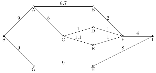
The size of  has to be appropriate for the situation. In the commercial vehicle routing program [16] all sections of a shortest (or fastest) route were multiplied by
  , i.e.,
  . Then the alternative route was computed. In [39] recognition of linear structures (streets, rivers, airport lanes) in satellite images was done by shortest path methods. Here
  turned out to be an appropriate choice for getting interesting alternative candidates.
Instead of relative penalty factors additive penalties might be used. That means we add a constant term  to all edges we want to punish. The only modification of the algorithm above is in step 4.

THEN
Example 23.2 Given is the graph  from Example 23.1 (see Figure 23.2). The shortest path from
  to
to  is still
  via
via  -
-  -
-  -
-  -
-  -
-  with length
  . Adding
  to all edges of
  and solving the resulting shortest path problem gives the alternative solution
  via
via  -
-  -
-  -
-  -
-  -
-  with modified length
  and normal length
  .
.  and
and  have three edges in common.
In principle this approach with additive penalties is not worse in comparison with multiplicative penalties. However, the method with multiplicative penalties has the advantage to be immune against artificial splits of edges.
For a generalisation of the penalty method from routing problems the following definition of optimisation problems is helpful.
Definition 23.1 Let  be an arbitrary finite set and
  a set of subsets of
  .
.  is called the base set and the elements of
  are feasible subsets of
  . Let
. Let  be a real valued weight function on
  . For every
  we set
  .
.
The optimisation problem  is a Sum Type Optimisation Problem or in short “
  -type problem”
Remarks:
-
The elements
 are also called feasible solutions.
 -
By substitution of
 by
by  every maximisation problem can be formulated as a minimisation problem. Therefore we will also call maximisation problems
  -type problems.
Examples of  -type problems
-
Shortest Path Problem
-
Assignment Problem
-
Travelling Salesperson Problem (TSP)
-
Knapsack Problem
-
Sequence Alignment Problem
Example 23.3 Consider the Knapsack Problem. Given a set of items  , a weight function
  , a value function
  , and a knapsack capacity
  . What is the most valuable collection of items whose weight sum does not exceed the knapsack capacity?
Choosing  as base set and
  as the family of all subsets whose weight sum is smaller or equal to
  gives a representation as a
  -type problem: maximise
  over all
  .
.
Abstract formulation of the penalty method for  -type problems
Definition 23.2 Let  be an arbitrary set and
  the set of feasible subsets of
  . Let
. Let  be a real-valued and
  a non-negative real-valued function on
  .
.
For every  , let
, let  be one of the optimal solutions of the problem


With an algorithm which is able to solve the unpunished problem  we can also find the solutions
  . We just have to modify the function
  by replacing
  by
by 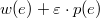 for all
  .
.  is called an
  penalty solution or an
  alternative.
Additionally we define the solution  of the problem

which has a minimal value  and among all such solutions a minimal value
  .
.
Remark. If both  and
and  are positive real-valued functions, there is a symmetry in the optimal solutions:
  is an
is an  penalty solution (
 ) for the function pair
  , if and only if
  is a
is a  penalty solution for the pair
  .
.
To preserve this symmetry it makes sense to define  as an optimal solution of the problem
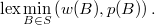
That means  is not only an optimal solution for the objective function
  , but among all such solutions it has also a minimal
  -value.
Example 23.4 We formulate the concrete Example 23.1 in this abstract  -type formulation. We know the shortest path
  from
from  to
to  and search for a “good” alternative solution. The penalty function
  is defined by
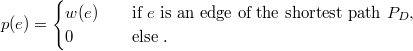
 .
.Often it is a priori not clear which choice of the penalty parameter  produces good and interesting alternative solutions. With a “divide-and-conquer” algorithm one is able to find all solutions which can be produced by any parameter
  .
.
For finite sets  we give an efficient algorithm which generates a “small” set
  of solutions with the following properties.
-
For each element
 there exists an
  such that
  is an optimal solution for the penalty parameter
  .
. -
For each
 there exists an element
  such that
  is optimal for the penalty parameter
  .
. -
 has a minimal number of elements among all systems of sets which have the two properties above.
We call a solution  which is optimal for at least one penalty parameter penalty-optimal. The following algorithm finds a set of penalty-optimal solutions which covers all
  .
.
For easier identification we arrange the elements of the set  in a fixed order
  , with
  .
.
The algorithm has to check that for  there is no
  with
with  such that for this penalty parameter
  neither
  nor
nor  is optimal. Otherwise it has to identify such an
  and an
  -penalty solution
  . In step 11 of the pseudo code below the variable Border
  is set to
  if it turns out that such an intermediate
  does not exist.
We present the pseudocode and give some remarks.
Algorithm for finding a sequence  of penalty-optimal solutions covering all
  for the problem
Divide-and-Cover(
)
1 compute, which minimises
and has a
-value as small as possible. 2 compute
, which minimises
and has a
-value as small as possible. 3
IF4
THEN;
; Border
(
minimises the functions
and
and is optimal for all
.) 5
ELSE;
; Border
;
. 6
WHILEThere is anwith Border
. 7
DO8 Find an optimal solution
for the parameter
. 9
IF10
THENBorder11
ELSE12
13 Border
(Border
,Border
Border
,
, Border
) 14
15
RETURN, Border
At the end  is a sequence of different penalty-optimal solutions and the vector
  includes consecutive epsilons.
This algorithm is based on the following properties:
-
(1) If
 is an
is an  -optimal solution then there exists an interval
  ,
,  , such that
  is optimal for all penalty parameters
  and for no other parameters.
 -
(2) For two different solutions
 and
and  with nonempty optimality intervals
  and
and  , only three cases are possible.

 . This happens iff
  and
and  .
.

 and
and  are disjoint.

 , this means the intersection contains only a single epsilon. This happens if
  and
and  are neighbouring intervals.
By finiteness of  there are only finitely many feasible solutions
  . So, there can be only finitely many optimality intervals. Hence, (1) and (2) show that the interval
  can be decomposed into a set of intervals
  . For each interval we have a different solution
  which is optimal for all
  in this interval. We call such a solution an interval representative.
-
(3) The aim of the algorithm is to find the borders of such optimality intervals and for each interval a representing solution. In every iteration step an interval representative of a new interval or a new border between two different intervals will be found (in steps 7–13). When there are
 optimality intervals with
  it is sufficient to solve
  problems of the type
  to detect all of them and to find representing solutions.
When only one  -alternative shall be computed the question comes up which penalty parameter should be used to produce a “best possible” alternative solution. If the penalty parameter is too small the optimal and the alternative solution are too similar and offer no real choice. If the parameter is too large the alternative solution becomes too poor. The best choice is to take some “medium”
  .
.
We illustrate this effect in the following route planning example.
Example 23.5 Assume that we have to plan a route from a given starting point to a given target. We know the standard travel times of all road sections and are allowed to plan for two different routes. In last minute we learn about the real travel times and can choose the fastest of our two candidate routes.
Let the first route be the route with the smallest standard travel time and the second one a route found by the penalty method. Question: Which penalty parameter should we use to minimise the real travel time of the fastest route?
Concretely, consider randomly generated instances of the shortest path problem in a weighted directed grid graph  of dimension
  . The weights of the arcs are independently uniformly distributed in the unit interval
  . We compute
  , a path from the lower left corner to the upper right with minimal weight. Afterwards we punish the edges of path
  by multiplying by
  and calculate a whole set of
  -penalty solutions
 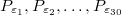 for
for  . We get 30 solution pairs
  and can compare these.
The weight  of an arc
  is the standard travel time without time lags, i.e. the minimal needed travel time on a free road without any traffic jam. The real travel time
  of this arc may differ from
  as follows:
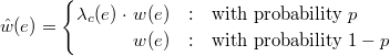
independently for all edges  . Here the
  are independent random numbers, uniformly distributed in the interval
  . The parameter
  is called failure probability and the parameter
  is called failure width.
For every pair  we calculate the minimum of the two function values
  and
and  . To get a direct impression of the benefit of having two solutions instead of one we scale with respect to the real value of the optimal solution
  .
.
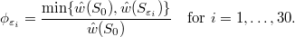
We computed the values  for 100,000 randomly generated
  grid graphs with failure probability
  and failure width
  . Figure 23.3 shows the averages
  for
for  .
.
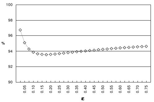
As seen in Figure 23.3, the expected quality  of the solution pairs is unimodal in
  . That mean that
  first decreases and then increases for growing
  . In this example
  is the optimal penalty parameter.
In further experiments it was observed that the optimal parameter  is decreasing in the problem size (e.g.
  for shortest paths in
  -grids,
  for
for  and
and  for
for  grid graphs).
Independently whether all  -penalty solutions are generated or only a single one (as in the prevoius pages), the following structural properties are provable: With increasing penalty factor
  we get solutions
  where
where
-
the penalty part
 of the objective function is fitted monotonically better (the solution contains less punished parts),
 -
the original objective function
 is getting monotonically worse, in compensation for the improvement with respect to the penalty part.
These facts are formalised in the following theorem.
Theorem 23.3 Let  be a real-valued function and
  a positive real-valued function on
  . Let
. Let  be defined for
  according to Definition 23.2. The following four statements hold:
(i)  is weakly monotonically decreasing in
  .
.
(ii)  is weakly monotonically increasing in
  .
.
(iii) The difference  is weakly monotonically increasing in
  .
.
(iv)  is weakly monotonically increasing in
  .
.
Proof. Let  and
and  be two arbitrary nonnegative real numbers with
  .
.
Because of the definition of  and
and  the following inequalities hold.
(i) In case  we have


Subtracting (23.2) from (23.1) we get


In case  inequality (23.3) follows directly from the definition of
  .
.
(ii) Subtracting (23.3) multiplied with  from (23.2) we get

(iii) Subtracting (23.3) from (23.4) we get

(iv) With (23.2) and  we have


 .
.If we have a solution  and want to get more than one alternative solution we can use the penalty method several times by punishing
  with different penalty parameters
  , getting alternative solutions
  . This method has a big disadvantage, because only the shared parts of the main solution
  and each alternative solution are controlled by the values
  . But there is no direct control of the parts shared by two different alternative solutions. So,
  and
and  may be rather similar for some
  .
.
To avoid this effect the penalty method may be used iteratively for the same  .
.
Iterative-Penalty-Method(
)
1 solve the original problemand find the optimal solution
. 2 define the penalty function as
. 3 solve the modified problem
and find the solution
. 4
FOR
TO5
DO6 solve the modified problem
and find the solution
. 7
RETURN
Step 5 may be replaced by the variant 

DO

In the first case (5) a part of a solution belonging to  of the
  solutions
  and
and  is punished by the factor
  . In the second case (
 ) a part of a solution is punished with multiplicity one if it belongs to at least one of
  or
or  .
.
The differences in performance are marginal. However, in shortest path problems with three solutions  and
and  setting (5) seemed to give slightly better results.
Example 23.6 Take the graph  from Figure 23.2. For penalty parameter
  we want to find three solutions. The shortest path from
  to
to  is
is  via
via  -
-  -
-  -
-  -
-  -
-  with length
  . Multiplying all edges of
  by
by  and solving the obtained shortest path problem gives the alternative solution
  via
via  -
-  -
-  -
-  -
-  .
.
Applying setting  we have to multiply the edge lengths of
  ,
,  ,
,  ,
,  and
and  by penalty factor 1.1. The edges
  and
and  have to be multiplied by factor 1.2 (double penalty). The optimal solution is path
  via
via  -
-  -
-  -
-  .
.
Applying setting  we have to multiply the edge lengths
  ,
,  ,
,  ,
,  ,
,  ,
,  and
and  by penalty factor 1.1. The optimal solution of this modified problem is path
  via
via  -
-  -
-  -
-  -
-  -
-  .
.
It is well known that shortest path problems as well as many other network flow problems can be solved with Linear Programming. Linear Programming may also be used to generate alternative solutions. We start with the description of Linear Programming for the basic shortest path problem.
The shortest path problem formulated as a linear program.
Consider a directed graph  and a function
  assigning a length to every arc of the graph. Let
  and
and  be two distinguished nodes of
  .
.
Which is the shortest simple path from  to
to  in
in  ?
?
For every arc  we introduce a variable
  . Here
  shall be
  if
if  is part of the shortest path and
  shall be
  otherwise.
With  we denote the set of the successors of node
  and with
  we denote the set of the predecessors of node
  . The linear program
  is formulated as follows:
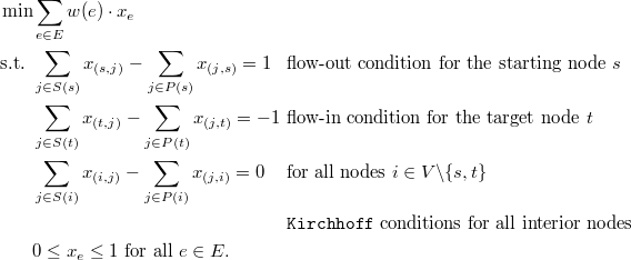
By the starting and target conditions node  is a source and node
  is a sink. Because of the
 Kirchhoff conditions there are no other sources or sinks. Therefore there must be a “connection” from  to
to  .
.
It is not obvious that this connection is a simple path. The variables  might have non-integer values or there could be circles anywhere. But there is a basic theorem for network flow problems [7][p. 318] that the linear program
 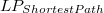 has an optimal solution where all
  have the value
  . The according arcs with
  represent a simple path from
  to
to  .
.
Example 23.7 Consider the graph in Figure 23.4. The linear program for the shortest path problem in this graph contains six equality constraints (one for each node) and seven pairs of inequality constraints (one pair for each arc).
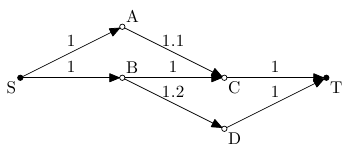
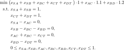
The optimal solution has  .
.
A linear program which gives two alternative paths from  to
to 
Here we give an  -representation for the task to find two alternative routes from
  to
to  .
.
For every arc  we introduce two variables
  and
and  . If the arc
  is used in both routes, then both
  and
and  shall have the value
  . If
. If  is a part of only one route,
  shall be
  and
and  shall be
  . Otherwise
  and
and  shall both be
  .
.  is a penalty parameter to punish arcs used by both routes.
With this in mind we can formulate the linear program 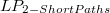
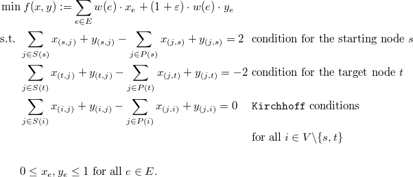
Example 23.8 Consider again the graph in Figure 23.4. The linear program for the  -alternative-paths problem in this graph contains six equality constraints (one for each node) and
  pairs of inequality constraints.
This linear program can be interpreted as a minimal cost flow problem.
Where is the connection between the linear program and the problem to find two candidate routes from  to
to  ?
?
Theorem 23.4 If the linear program  has an optimal solution then it has also an optimal solution
  with the following properties.
There are disjoint sets  with
with
(i)  ,
,  and
and  ,
,
(ii)  ,
,  for all
  ,
,
(iii)  ,
,  for all
  ,
,
(iv)  ,
,  for all
  .
.
(v)  represents a path P
  from
from  to
to  and
and  represents a path P
  from
from  to
to  .
.  is the set of arcs used by both paths.
(vi) No other pair  of paths is better than
  , i.e.,

That means the sum of the lengths of P  and P
and P  plus a penalty for arcs used twice is minimal.
We conclude with some remarks.
-
For each arc
 there are two variables
  and
and  . This can be interpreted as a street with a normal lane and an additional passing lane. Using the passing lane is more expensive than using the normal lane. If a solution uses an arc only once, it takes the cheaper normal lane. But if a solution uses an arc twice, it has to take both the normal and the passing lane.
 -
The decomposition of the solution
 into two paths from the starting node to the target node is in most cases not unique. With the arcs
  in Figure 23.4 we can build two different pairs of paths from
  to
to  , namely
  and
and  . Both pairs are equi-optimal in the sense of Theorem 23.4. So the user has the chance to choose between them according to other criteria.
 -
The penalty method and the LP-penalty method generally lead to different results. The penalty method computes the best single solution and a suitable alternative. The LP-penalty method computes a pair of good solutions with relatively small overlap. Figure 23.5 shows that this pair not necessarily contains the best single solution. The shortest path from
 to
to  is
is  –
–  –
–  –
–  with length
  . For all
  the
the  -penalty solution is
  –
–  –
–  –
–  . The path pair
  has a total lengths of
  and a shared length of
  . But for
  the LP-Penalty method produces the pair
  with a total length of
  and a shared length of zero.
 -
Finding
 candidate routes for some larger number
  is possible, if we introduce
  variables
  ,
,  for each arc
  and set the supply of
  and the demand of
  to
to  . As objective function we can use for instance
 -
The LP-penalty method does not only work for shortest path problems. It can be generalised to arbitrary problems solvable by linear programming.
-
Furthermore an analogous method – the Integer Linear Programming Penalty Method – can be applied to problems solvable by integer linear programming.
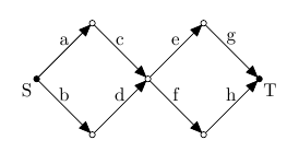
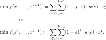
In Subsection 23.2.2 we discussed the penalty method in combination with exact solving algorithms (e.g. Dijkstra-algorithm or dynamic programming for the shortest path problem). But also in case of heuristics (instead of exact algorithms) the penalty method can be used to find multiple candidate solutions.
Example 23.9 A well known heuristic for the TSP-problem is local search with 2-exchange steps (see Subsection 23.2.1).
Penalty-Method-for-the-TSP-Problem-with-2-Exchange-Heuristic
1 apply the 2-exchange heuristic to the unpunished problem getting a locally (but
not necessarily globally) optimal solution  2 punish the edges belonging to
  by multiplying their lengths with
  3 apply the 2-exchange heuristic to the punished problem getting an alternative
solution
3 apply the 2-exchange heuristic to the punished problem getting an alternative
solution  4 compute the unmodified length of
  5 the pair
  is the output
Question: Which penalty parameter  should be used to minimise the travel time of the fastest route?
An experiment analogous to the one described in Example 23.5 was executed for TSP instances with  random cities in the unit square. Figure 23.6 shows the scaled averages for
  .
.
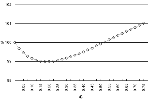
So, the expected quality  of the solution pairs is (again) unimodal in the penalty factor
  . That means that
  first decreases and then increases for growing
  . In this example
  is the optimal penalty parameter.
In further experiments it was observed that the optimal penalty parameter  is decreasing in the problem size.
Exercises
23.2-1 The following programming exercise on the Travelling Salesperson Problem helps to get a feeling for the great variety of local optima. Generate 200 random points in the 2-dimensional unit-square. Compute distances with respect to the Euclidean metric. Make 100 runs of local search with random starting tours and 2-exchanges. Count how many different local minima have been found.
23.2-2 Enter the same key words into different internet search engines. Compare the hit lists and their diversities.
23.2-3 Formulate the Travelling Salesperson Problem as a  -type problem.
23.2-4 Proof the assertion of the remark on page.
23.2-5 How does the penalty function  look like in case of additive penalties like in Example 23.2?
23.2-6 Prove the properties (1) and (2) after the algorithm Divide-and-Cover(
).
23.2-7 Apply the Divide and cover algorithm to the shortest path problem in Figure 23.2 with starting node  and target node
  . Set
. Set  length of
  for each road section, and
  length of
  for the road sections belonging to the shortest path
  via
via  -
-  -
-  -
-  -
-  -
-  and
and  for all other sections. So, the penalty value of a whole path is the length of this part shared with
  .
.
23.2-8 Find a penalty parameter  for Example 23.6 such that the first setting (5) produces three different paths but the second setting (
 ) only two different paths for
  .
.
There are many other settings where a human controller has access to computer-generated candidate solutions. This section lists four important cases and concludes with a discussion of miscellaneous stuff.
In an anytime-setting the computer starts to work on a problem, and almost from the very first moment on candidate solutions (the best ones found so far) are shown on the monitor. Of course, the early outputs in such a process are often only preliminary and approximate solutions – without guarantee of optimality and far from perfect.
An example: Iterative deepening performs multiple depth-limited searches – gradually increasing the depth limit on each iteration of the search. Assume that the task is to seek good solutions in a large rooted tree  . Let
. Let  be the function which is to be maximised. Let
  be the set of all nodes in the tree at distance d from root.
Iterative-Deepening-Tree-Search(
)
1 Opt2
3
WHILE4
DODetermine maximum Maxof
on
5
IFMaxOpt 6
THENOptMax
7

All the time the currently best solution (Opt) is shown on the monitor. The operator may stop at any moment.
Iterative deepening is not only interesting for HCI but has also many applications in fully automatic computing. A prominent example is game tree search: In tournament chess a program has a fixed amount of time for 40 moves, and iterative deepening is the key instrument to find a balanced distribution of time on the single alpha-beta searches.
Another frequent anytime scenario is repeated application of a heuristic. Let  be some complicated function for which elements with large function values are searched. Let
  be a probabilistic heuristic that returns a candidate solution for this maximisation problem
  . For instance,
  may be local search or some other sort of hill-climbing procedure.
  is applied again and again in independent runs, and all the time the best solution found so far is shown.
A third anytime application is in Monte Carlo simulations, for instance in Monte Carlo integration. A static approach would take objective values at a prescribed number of random points (1,000 or so) and give the average value in the output. However, already the intermediate average values (after 1, 2, 3 etc. data points – or after each block of 10 or 50 points) may give early indications in which region the final result might fall and whether it really makes sense to execute all the many runs. Additional display of variances and frequencies of outliers gives further information for the decision when best to stop the Monte Carlo run.
In human-computer systems anytime algorithms help also in the following way: during the ongoing process of computing the human may already evaluate and compare preliminary candidate solutions.
Genetic Algorithms are search algorithms based on the mechanics of natural selection and natural genetics. Instead of single solutions whole populations of solutions are manipulated. Genetic Algorithms are often applied to large and difficult problems where traditional optimisation techniques fall short.
Interactive evolution is an evolutionary algorithm that needs human interaction. In interactive evolution, the user selects one or more individual(s) of the current population which survive(s) and reproduce(s) (with mutations) to constitute the new generation. So, in interactive evolution the user plays the role of an objective function and thus has a rather active role in the search process.
In fields like art, architecture, and photo processing (including the design of phantom photos) Generative Design is used as a special form of interactive evolution. In Generative Design all solutions of the current generation are shown simultaneously on the screen. Here typically “all” means some small number  between 4 and 20. Think of photo processing as an example, where the user selects modified contrast, brightness, colour intensities, and sharpness. The user inspects the current candidate realizations, and by a single mouse click marks the one which he likes most. All other solutions are deleted, and
  mutants of the marked one are generated. The process is repeated (open end) until the user is happy with the outcome. For people without practical experience in generative design it may sound unbelievable, but even from poor starting solutions it takes the process often only a few iterations to come to acceptable outcomes.
Many problems are high-dimensional, having lots of parameters to adjust. If sets of good solutions in such a problem are generated by repeated probabilistic heuristics, the following interactive multi-stage procedure may be applied: First of all several heuristic solutions are generated and inspected by a human expert. This human especially looks for “typical” pattern in the solutions and “fixes” them. Then more heuristic solutions are generated under the side condition that they all contain the fixed parts. The human inspects again and fixes more parts. The process is repeated until finally everything is fix, resulting in one specific (and hopefully good) solution.
In multicriteria decision making not only one but two or more objective functions are given. The task is to find admissible solutions which are as good as possible with respect to all these objectives. Typically, the objectives are more or less contradictory, excluding the existence of a unanimous optimum. Helpful is the concept of “efficient solutions”, with the following definition: For an efficient solution there exists no other solution which is better with respect to at least one objective and not worse with respect to all the others.
A standard first step in multicriteria decision making is to compute the set of all efficient solutions. In the bicriteria case the “efficient frontier” can be visualized in a 2-dimensional diagram, giving the human controller a good overview of what is possible.
-
Graphical Visualisation of Computer Solutions
It is not enough that a computer generates good candidate solutions. The results also have to be visualized in appropriate ways. In case of a single solution important parts and features have to be highlighted. And, even more important, in case of concurring solutions their differences and specialities have to be stressed.
-
Permanent Computer Runs with Short Intermediate Human Control
A nickname for this is “1+23h mode”, coming from the following picture: Each day the human sits in front of the computer for one hour only. In this hour he looks at the computer results from the previous 23 hours, interacts with the machine and also briefs the computer what to do in the next 23 hours. So, the human invests only a small portion of his time while the computer is running permanently.
An impressive example comes from correspondence chess. Computer help is officially permitted. Most top players have one or several machines running all around the clock, analysing the most critical positions and lines of play. The human players collect these computer results and analyse only shortly per day.
-
Unexpected Errors and Numerical Instabilities
“Every software has errors!” This rule of thumb is often forgotten. People too often simply believe what the monitor or the description of a software product promises. However, running independent programs for the very same task (with a unique optimal solution) will result in different outputs unexpectedly often. Also numerical stability is not for free. Different programs for the same problem may lead to different results, due to rounding errors. Such problems may be recognised by applying independent programs.
Of course, also hardware has (physical) errors, especially in times of ongoing miniaturisation. So, in crucial situations it is a good strategy to run an identical program on fully independent machines - best of all operated by independent human operators.
Exercises
23.3-1 For a Travelling Salesperson Problem with 200 random points  in the unit square
  and Euclidean distances, generate 100 locally optimal solutions (with 2-exchanges, see Subsection 23.2.1) and count which edges occur how often in these 100 solutions. Define some threshold
  (for instance
  ) and fix all edges which are in at least
  of the solutions. Generate another 100 local optima, without allowing the fixed edges to be exchanged. Repeat until convergence and compare the final result with typical local optima from the first series.
CHAPTER NOTES |
In the technical report [293] lots of experiments on the penalty method for various sum type problems, dimensions, failure widths and probabilities are described and analysed. The proof of Theorem 23.3 was originally given in [13]). In e-commerce multiple-choice systems are often called “Recommender Systems” [285], having in mind customers for whom interesting products have to be listed. Understandably, commercial search engines and e-companies keep their shortlisting strategies secret.
A good class book on Genetic Algorithms is [134]. Interactive Evolution and Generative Design are described in [30]. There is a lot of literature on multicriteria decision making, one of the standard books being [123].
In the book [10] the story of 3-Hirn and its successes in tournament chess is told. The final match between “3-Hirn” and GM Yussupov is described in [12]. [11] gives more general information on improved game play by multiple computer hints. In [14] several good  -best realizations of iterative deepening in game tree search are exhibited and discussed. Screenshots of these realizations can be inspected at http://www.minet.uni-jena.de/www/fakultaet/iam/personen/k-best.html. [161] describes the technical background of advanced programs for playing chess and other games.
There is a nice online repository, run by M. Zuker and D.H. Turner at http://www.bioinfo.rpi.edu/applications/mfold/. The user may enter for instance RNA-strings, and in realtime alternative foldings for these strings are generated. Amongst other data the user may enter parameters for “maximum number of computed foldings” (default = 50) and “percent suboptimality number” (default = 5 %).
[1] Querying semi-structured data, Lecture Notes in Computer Science, In F. Afrati, P. Kolaitis(Eds.) Proceedings of ICDT'97. Springer-Verlag. 1997. 1–18.
[2] Complexity of answering queries using materialized views, In Proceedings of the Seventeenth ACM SIGACT-SIGMOD-SIGART Symposium on Principles of Database Systems. ACM-Press. 1998. 254–263.
[3] Foundations of Databases. Addison-Wesley. 1995.
[4] Ancestral Maximum Likelihood of Phylogenetic Trees is Hard. Lecture Notes in Bioinformatics. 2003. 202–215.
[5] Broadband Traffic Modeling: Simple Solutions to Hard Problems. IEEE Communications Magazine. 1998. 88–95.
[6] The theory of joins in relational databases. ACM Transactions on Database Systems. 1979. 297–314.
[7] Network Flows: Theory, Algorithms, and Applications. Prentice Hall. 1993.
[8] Dynamic programming algorithms for RNA secondary prediction with pseudoknots. Discrete Applied Mathematics. 2000. 45–62.
[9] Multiple sequence alignment with arbitrary gap costs: Computing an optimal solution using polyhedral combinatorics. Bioinformatics. 2002. S4–S16.
[10] 13 Jahre 3-Hirn. Published by the author. 1998.
[11] Improved game play by multiple computer hints. Theoretical Computer Science. 2004. 315–324.
[12] List-3-Hirn vs. Grandmaster Yussupov – report on a very experimental match. ICCA Journal. 1998. 52–60 and 131–134.
[13] Generating True Alternatives with a Penalty Method. http://www.minet.uni-jena.de/Math-Net/reports/shadows/02-04report.html. 2002.
[14] Five visualisations of the  -best mode. ICCA Journal. 2003. 182–189.
[15] Validity of the single-processor approach to achieving large-scale computer capabilities, In AFIPS Conference Proceedings. 1967. 483–485.
[17] Stochastic theory of a data handling system with multiple sources. The Bell System Technical Journal. 1982. 1871–1894.
[18] A normal form for XML documents, In Proceedings of the 21st Symposium on Principles of Database Systems. 2002. 85–96.
[19] On economic construction of the transitive closure of a directed graph. Doklady Academii Nauk SSSR. 1970. 487–488.
[20] Dependency structures of database relationships, In Proceedings of IFIP Congress. North Holland. 1974. 580–583.
[21] Eight open problems in distributed computing. Bulletin of European Association of Theoretical Computer Science of EATCS. 2006. 109–126.
[22] The performance of the neighbor-joining method of phylogeny reconstruction. Algorithmica. 1999. 251–278.
[23] Bounds on the time to reach agreement in the presence of timing uncertainty. Journal of the ACM. 1994. 122–142.
[24] Distributed Computing, Fundamentals, Simulations and Advanced Topics. McGraw-Hill. 1998.
[25] Complexity of network synchronization. Journal of the ACM. 1985. 804–823.
[26] Sorting by weighted reversals, transpositions and inverted transpsitions. Lecture Notes in Bioinformatics. 2006. 563–577.
[27] A tight asymptotic bound for next-fit decreasing bin-packing. SIAM Journal on Algebraic and Discrete Methods. 1981. 147–152.
[30] Interactive evolution, In T. Back, D. B. Fogel, Z. Michalewicz, T. Baeck (Eds.) Handbook of Evolutionary Computation. IOP Press. 1997.
[31] On the membership problem for functional and multivalued dependencies in relational databases. ACM Transactions on Database Systems. 1980. 241–259.
[32] Computational problems related to the design of normal form relational schemas. ACM Transactions on Database Systems. 1979. 30–59.
[33] On the structure of Armstrong relations for functional dependencies. Journal of ACM. 1984. 30–46.
[34] A complete axiomatization for functional and multivalued dependencies, In ACM SIGMOD Symposium on the Management of Data. 1977. 47–61.
[36] Empirical and structural models for insertions and deletions in the divergent evolution of proteins. Journal of Molecular Biology. 1993. 1065–1082.
[37] Statistics for Long-Memory Processes, Monographs on Statistics and Applied Probability. Chapman & Hall. 1986.
[38] Long-range dependence in variable-bit-rate video traffic. IEEE Transactions on Communications. 1995. 1566–1579.
 alternatives instead of
  shortest path.
 [40] Cloture votes: $n/4$-resilient distributed consensus in $t+1$ rounds. Mathematical Systems Theory. 1993. 3–19.
[42] Contribution to the theory of data base relations. Discrete Mathematics. 1979. 1–10.
[43] An anomaly in space-time characteristics of certain programs running in paging machine. Communications of the ACM. 1969. 349–353.
[44] A generalization of algebraic surface drawing. ACM Transactions on Graphics. 1982. 135–256.
[45] Introduction to Implicit Surfaces. Morgan Kaufmann Publishers. 1997.
[46] Linear approximation of shortest superstrings, In Proceedings of the 23rd ACM Symposium on Theory of Computing. 1991. 328–336.
[47] The Parallel Evaluation of General Arithmetic Expressions. Journal of the ACM. 1974. 201–206.
[48] Algorithm for Computer Control of a Digital Plotter. IBM Systems Journal. 1965. 25–30.
[49] Semistructured data, In Proceedings of the Sixteenth ACM SIGACT-SIGMOD-SIGART Symposium on Principles of Database Systems. ACM-Press. 1997. 117–121.
[50] UnQL: a query language and algebra for semistructured data based on structural recursion. The International Journal on Very Large Data Bases. 2000. 76–110.
[51] A formal model for message passing systems. Technical reports91, Indiana University. 1980.
[52] Bounds on shared memory for mutual exclusion. Information and Computation. 1993. 171–184.
[54] Answering regular path queries using views, In Proceedings of the Sixteenth International Conference on Data Engineering. 2000. 190–200.
[55] Formulations and complexity of multiple sorting by reversals, In RECOMB-99. ACM-Press. 1999. 84–93.
[56] Sorting Permutations by Reversals and Eulerian Cycle Decompositions. SIAM Journal on Discrete Mathematics. 1999. 91–110.
[57] The multiple sequence alignment problem in biology. SIAM Journal on Applied Mathematics. 1988. 1073–1082.
[58] Parallel Algorithms. Chapman & Hall. 2009.
[59] Recursively generated B-spline surfaces on arbitrary topological meshes. Computer-Aided Design. 1978. 350–355.
[60] Parallel Programming in OpenMP. Morgan Kaufmann Publishers. 2000.
[61] Optimizing queries with materialized views, In Proceedings of the Eleventh International Conference on Data Engineering. 1995. 190–200.
[62] Triangulating a Simple Polygon in Linear Time. Discrete and Computational Geometry. 1991. 353–363.
[63] An adaptive structural summary for graph-structured data, In Proceedings of the 2003 ACM SIGMOD International Conference on Management of Data. 2003. 134–144.
[64] Maximum likelihood of evolutionary trees: hardness and approximation. Bioinformatics. 2005. i97–i106.
[65] Sorting permutations by block-interchanges. Information Processing Letters. 1996. 165–169.
[66] A relational model of large shared data banks. Communications of the ACM. 1970. 377–387.
[67] Further normalization of the data base relational model, In R. Rustin Courant Computer Science Symposium 6: Data Base Systems. Prentice Hall. 1972. 33–64.
[68] Normalized database structure: A brief tutorial, In ACM SIGFIDET Workshop on Data Description, Access and Control. 1971. 24–30.
[69] Recent investigations in relational data base systems, In Information Processing 74. North-Holland. 1974. 1017–1021.
[70] Relational completeness of database sublanguages, In R. Rustin(Ed.) Courant Computer Science Symposium 6: Data Base Systems. Prentice Hall. 1972. 65–98.
[71] Computer and Job Shop Scheduling. John Wiley & Sons. 1976.
[72] Introduction to Algorithms. The MIT Press/McGraw-Hill. 1990.
[73] Introduction to Algorithms (3rd edition, second corrected printing). The MIT Press/McGraw-Hill. 2010.
[74] An efficient algorithm for graph isomorphism. Journal of the ACM. 1970. 51–64.
[75] Multiple sequence alignment with hierarchical clustering. Nucleic Acids Research. 1988. 10881–10890.
[77] Self-Similarity in World Wide Web Traffic: Evidence and Possible Causes. IEEE/ACM Transactions on Networking. 1997. 835–846.
[78] LogP: A practical model of parallel computation. Communication of the ACM. 1996. 78–85.
[79] Scheduling and Automatic Parallelization. Birkhuser Boston. 2000.
[80] A model of evolutionary change in proteins. Atlas of Protein Sequence and Structure. 1978. 345–352.
[82] Computational Geometry: Algorithms and Applications. Springer-Verlag. 2000.
[83] Normalization and hierarchical dependencies in the relational data model. ACM Transactions on Database Systems. 1978. 201–222.
[84] Minimal Representations of Branching Dependencies. Discrete Applied Mathematics. 1992. 139–153.
[85] Minimal Representations of Branching Dependencies. Acta Scientiarum Mathematicorum (Szeged). 1995. 213–223.
[86] Design type problems motivated by database theory. Journal of Statistical Planning and Inference. 1998. 149–164.
[87] Virtual memory. Computing Surveys. 1970. 153–189.
[89] Physical data independence, constraints and optimization with universal plans, In Proceedings of VLDB'99. 1999. 459–470.
[90] Authenticated algorithms for Byzantine agreement. SIAM Journal on Computing. 1983. 656–666.
[91] Large deviation and overflow probabilities for the general single-server queue, with applications. Mathematical Proceedings of the Cambridge Philosophical Society. 1995. 363–374.
[92] Statistical analysis of CCSN/SS7 traffic data from working CCS subnetworks. IEEE Journal on Selected Areas Communications. 1994. 544–551.
[93] Answering recursive queries using views, In Proceedings of the Sixteenth ACM SIGACT-SIGMOD-SIGART Symposium on Principles of Database Systems. ACM-Press. 1997. 109–116.
[94] Query planning in infomaster, In Proceedings of ACM Symposium on Applied Computing. ACM-Press. 1997. 109–111.
[95] A butterfly subdivision scheme for surface interpolation with tension control. ACM Transactions on Graphics. 1990. 160–169.
[96] A 1.375 approximation algorithm for sorting by transpositions. Lecture Notes in Bioinformatics. 2005. 204–215.
[98] Local quartet splits of a binary tree infer all quartet splits via one dyadic inference rule. Computers and Artificial Intelligence. 1997. 217–227.
[99] Experimental queueing analysis with long-range dependent packet-traffic. IEEE/ACM Transactions on Networking. 1996. 209–223.
[100] Armstrong databases, In Proceedings of IBM Symposium on Mathematical Foundations of Computer Science. 1982. 24 pages.
[101] Horn clauses and database dependencies. Journal of ACM. 1982. 952–985.
[102] Multivalued dependencies and a new normal form for relational databases. ACM Transactions on Database Systems. 1977. 262–278.
[103] Curves and Surfaces for Computer Aided Geometric Design. Morgan Kaufmann Publishers. 2002 (2nd revised edition).
[104] Evolutionary trees from DNA sequences: a maximum likelihood approach. Journal of Molecular Evolution. 1981. 368–376.
[105] Progressive sequence alignment as a prerequisite to correct phylogenetic trees. Journal of Molecular Evolution. 1987. 351–360.
[106] GPUGems: Programming Techniques, Tips, and Tricks for Real-Time Graphics. Addison-Wesley. 2004.
[107] Fast optimal alignment. Nucleid Acids Research. 1984. 175–180.
[108] Impossibility of distributed consensus with one faulty proces. Journal of the ACM. 1985. 374–382.
[109] Toward defining the course of evolution: minimum change for a specified tree topology. Systematic Zoology. 1971. 406–416.
[112] Answering queries using OQL view expressions, In Workshop on Materialized views, in cooperation with ACM SIGMOD. 1996. 627–638.
[113] Very high-speed computer systems. Proceedings of the IEEE. 1966. 1901–1909.
[114] Computer Graphics: Principles and Practice. Addison-Wesley. 1990.
[115] Bélády's anomaly is unbounded In E. Kovács, Z. Winkler (Eds.) 5th International Conference on Applied Informatics. Molnár és társa. 2002. 65–72.
[116] Parallelism in Random Access Machines, In Proceedings of the Tenth Annual ACM Symposium on Theory of Computing. 1978. 114–118.
[117] The Grid: Blueprint for a New Computing Infrastructure. Morgan Kaufman Publisher. 2004 (2nd edition).
[118] The Physiology of the Grid: An Open Grid Services Architecture for Distributed Systems Integration. Available at www.globus.org/research/papers/ogsa.pdf. 2002.
[119] The Steiner problem in phylogeny is NP-complete. Advances in Applied Mathematics. 1982. 43–49.
[120] Efficient execution of information gathering plans, In Proceedings International Joint Conference on Artificial Intelligence. 1997. 785–791.
[121] On Visible Surface Generation by A Priory Tree Structures, Computer Graphics (SIGGRAPH '80 Proceedings). 1980. 124–133.
[122] ARTS: Accelerated Ray-Tracing System. IEEE Computer Graphics and Applications. 1986. 16–26.
[123] Multicriteria Decision Making. Kluwer Academic Publisher. 1999.
[124] Speeding up dynamic programming with applications to molecular biology. Theoretical Computer Science. 1989. 107–118.
[125] On finding minimal length superstrings. Journal of Computer and System Sciences. 1980. 50–58.
[126] Proofs that yield nothing but their validity or all languages in NP. Journal of the ACM. 1991. 691–729.
[127] Elections in a distributed computing systems. IEEE Transactions on Computers. 1982. 47–59.
[128] Computers and Intractability: A Guide to the Theory of NP-Completeness. W. H. Freeman. 1979.
[129] Bounds for sorting by prefix reversals. Discrete Mathematics. 1979. 47–57.
[130] Compatible sequences and a slow Winkler percolation. Combinatorics Probability and Computing. 2004. 815–856.
[131] Algebraic Theory of Automata. Akadémiai Kiadó. 1972.
[132] Can a shared-memory model serve as a bridging model for parallel computation. Theory of Computing Systems. 1999. 327–359.
[133] An Introduction to Ray Tracing. Academic Press. 1989.
[134] Genetic Algorithms in Search, Optimization, and Machine Learning. Addison-Wesley. 1989.
[135] Using evolutionary trees in protein secondary structure prediction and other comparative sequence analyses. Journal of Molecular Biology. 1996. 196–208.
[136] Optimizing queries using materialized views: a practical, scalable solution, In Optimizing queries using materialized views: a practical, scalable solution. 2001. 331–342.
[138] An improved algorithm for matching biological sequences. Journal of Molecular Biology. 1982. 705–708.
[139] The complexity of XPath query evaluation, In Proceedings of the 22nd Symposium on Principles of Database Systems. 2003. 179–190.
[140] Tableau techniques for querying information sources through global schemas, Lecture Notes in Computer Science., In Proceedings of ICDT'99. Springer-Verlag. 1999. 332–347.
[141] Introduction to Parallel Computing. Addison-Wesley. 2003 (2nd edition).
[142] Inferences for numerical dependencies. Theoretical Computer Science. 1985. 271–287.
[143] Normalization and axiomatization for numerical dependencies. Information and Control. 1985. 1–17.
[144] Notes on database operating system, In R. Bayer, R. M. Graham, G. Seegmuller (Eds.) Operating Systems: An Advanced Course, Lecture Notes in Computer Science. Springer-Verlag. 1978. 393–481.
[145] MPI: The Complete Reference, Scientific and Engineering Computation Series. The MIT Press. 1998.
[146] A 2-Approximation Algorithm for Genome Rearrangements by Reversals and Transpositions. Theoretical Computer Science. 1999. 327–339.
[147] A measurement study of diskless workstation traffic on an Ethernet. IEEE Transactions on Communications. 1990. 1557–1568.
[148] Algorithms on Strings, Trees and Sequences. Cambridge University Press. 1997.
[149] Efficient methods for multiple sequence alignment with guaranteed error bounds. Bulletin of Mathematical Biology. 1993. 141–154.
[150] Reevaluating Amdahl's law. Communications of ACM. 1988. 532–535.
[151] Simulation of the Harmful Consequences of Self-Similar Network Traffic. The Journal of Computer Information Systems. 2002. 94–111.
[152] Extension of multiprotocol label switching for long-range dependent traffic: QoS routing and performance in IP networks. Computer Standards and Interfaces. 2005. 117–132.
[153] Answering queries using views: A survey. The VLDB Journal. 2001. 270–294.
[154] Logic based techniques in data integration, In J. Minker Logic-based Artificial Intelligence. Kluwer Academic Publishers. 2000. 575–595.
[155] Answering queries using views, In Proceedings of the Fourteenth ACM SIGACT-SIGMOD-SIGART Symposium on Principles of Database Systems. ACM-Press. 1995. 95–104.
[156] Querying heterogeneous information sources using source descriptions, In Proceedings of Very Large Data Bases. 1996. 251–262.
[157] Polynomial-time algorithm for computing translocation distance between genomes. Discrete Applied Mathematics. 1996. 137–151.
[159] Multiresolution indexing of XML for frequent queries, In Proceedings of the 20th International Conference on Data Engineering. 2004. 683–694.
[160] A Markov modulated characterization of packetized voice and data traffic and related statistical multiplexer performance. IEEE Journal on Selected Areas in Communication. 1986. 856–868.
[161] Algorithmic Enhancements and Experiments at High Search Depths. Algorithmic Enhancements and Experiments at High Search Depths. 2000.
[162] Computing simulations on finite and infinite graphs, In Proceedings of the 36th Annual Symposium on Foundations of Computer Science. IEEE Computer Society Press. 1995. 453–462.
[163] The Use of Projective Geometry in Computer Graphics. Springer-Verlag. 1991.
[164] Principia Cybernetica Project. http://pespmc1.vub.ac.be/HEYL.html. 2004.
[165] A linear space algorithm for computing maximal common subsequences. Communications of the ACM. 1975. 341–343.
[166] Introduction to Automata Theory, Languages, and Computation. Addison-Wesley. 2001. (2nd edition).
[168] Local similarity in RNA secondary structure, In Proceedings of IEEE Bioinformatics Conference 2003. 2003. 159–168.
[170] Hidden Markov models for sequence analysis: Extension and analysis of the basic method. CABIOS. 1996. 95–107.
[171] A fast algorithm for computing longest common subsequences. Communications of the ACM. 1977. 350–353.
[172] Scalable Parallel Computing. McGraw-Hill. 1998.
[173] http://wwww.interoute.com/glossary.html. 2004.
[174] Density of safe matrices. Acta Universitatis Sapientiae. 2009. 121–142.
[175] On dumpling-eating giants, Colloquia of Mathematical Society János Bolyai, In Finite and Infinite Sets (Eger, 1981). North-Holland. 1984. 279–390.
[176] Párhuzamos algoritmusok (Parallel Algorithms). ELTE Eötvös Kiadó. 2003.
[177] Performance bounds for simple bin packing algorithms. Annales Universitatis Scientiarum Budapestinensis de Rolando Eötvös Nominatae, Sectio Computarorica. 1984. 77–82.
[178] Tight worst-case bounds for bin packing algorithms, Colloquia of Mathematical Society János Bolyai, In Theory of Algorithms (Pécs, 1984). North-Holland. 1985. 233–240.
[179] Elements of Theoretical Programming (in Russian). Moscow State University. 1985.
[180] Packet trains: Measurements and a new model for computer network traffic. IEEE Journal on Selected Areas in Communication. 1986. 986–995.
[181] The complexity of finding minimum-length generator sequences. Theoretical Computer Science. 1986. 265–289.
[183] 3D Collision Detection: A Survey. Computers and Graphics. 2001. 269–285.
[184] Near-Optimal Bin Packing Algorithms. MIT Department of Mathematics. 1973.
[185] Worst-case performance-bounds for simple one-dimensional bin packing algorithms. SIAM Journal on Computing. 1974. 299–325.
[186] Consultant's Guide to COMNET III. CACI Product Company. 1997.
[187] Information and Coding Theory. Springer-Verlag. 2000.
[188] Compiler algorithms for optimizing locality and parallelism on shared and distributed-memory machines. Journal of Parallel and Distributed Computing. 2000. 924–965.
[189] A First Course in Stochastic Processes. Academic Press. 1975.
[190] The organization of computations for uniform recurrence equations. Journal of the ACM. 1967. 563–590.
[191] Covering indexes for branching path queries, In Proceedings of the 2002 ACM SIGMOD International Conference on Management of Data. 2002. 133–144.
[193] Exploiting local similarity for indexing paths in graph-structured data, In Proceedings of the 18th International Conference on Data Engineering. 2002. 129–140.
[194] On the integration of structure indexes and inverted lists, In Proceedings of the 2004 ACM SIGMOD International Conference on Management of Data. 2004. 779–790.
[195] A polyhedral approach to sequence alignment problems. Discrete Applied Mathematics. 2000. 143–186.
[197] Optimizing Compilers for Modern Architectures. Morgan Kaufman Publishers. 2001.
[198] Encyclopedia of Information Science and Technology, Vol. 1, Vol. 2, Vol. 3, Vol. 4, Vol. 5. Idea Group Inc.. 2005.
[199] Programming with Threads. Prentice Hall. 1996.
[200] Queueing Systems. John Wiley & Sons. 1975.
[201] Pfold: RNA secondary structure prediction using stochastic context-free grammars. Nucleic Acids Researchs. 2003. 3423–3428.
[202] RNA secondary structure prediction using stochastic context free grammars and evolutionary history. Bioinformatics. 1999. 446–454.
[203] Fast pattern matching in strings. SIAM Journal on Computing. 1977. 323–350.
[204] The High Performance Fortran Handbook. The MIT Press. 1994.
[205] Notes on the Mathematics of the PHIGS Output Pipeline. Computer Graphics Forum. 1989. 219–226.
[206] Distributed Computing. Cambridge University Press. 2008.
[207] Systolic arrays (for VLSI), In I. S. Duff, G. W. Stewart (Eds.) Sparse Matrix Proceedings. SIAM. 1978. 256–282.
[208] Planning to gather information, In Proceedings of AAAI 13th National Conference on Artificial Intelligence. 1996. 32–39.
[209] Anomalies in parallel branch and bound algorithms. Communications of ACM. 1984. 594–602.
[210] Optimizing recursive information gathering plans, In Proceedings of 16th International Joint Conference on Artificial Intelligence. 1999. 1204–1211.
[211] Stochastic Processes. Springer-Verlag. 1972.
[212] A new solution of Dijkstra's concurrent programming problem. Communications of the ACM. 1974. 453–455.
[214] The Byzantine generals problem. ACM Transactions on Programming Languages and Systems. 1982. 382–401.
[215] Integer programming models for computational biology problems. Journal of Computer Science and Technology. 2004. 60–77.
[216] Eficient string matching with  mismatches. Theoretical Computer Science. 1986. 239–249.
[217] Simulation Modeling and Analysis. 3rd edition, McGraw-Hill Higher Education. 1976.
[218] Introduction to Parallel Algorithms and Architectures: Arrays-Trees-Hypercubes. Morgan Kaufman Publishers. 1992.
[219] Introduction to Parallel Algorithms and Architectures: Algorithms and VSLI. Morgan Kaufman Publishers. 2001.
[220] On the self-similar nature of Ethernet traffic. Computer Communication Reviews. 1993. 183–193.
[221] Parallel and Distributed Computing, Wiley Series on Parallel and Distributed Computing. John Wiley & Sons. 2001.
[222] Multithreaded Programming with Phtreads. Prentice Hall. 1998.
[224] Architectural and Technological Issues for Future Optical Internet Networks. IEEE Communications Magazine. 2000. 82–92.
[226] Bayesian phylogenetic inference under a statistical indel model. Lecture Notes in Bioinformatics. 2003. 228–244.
[227] An efficient algorithm for statistical multiple alignment on arbitrary phylogenetic trees. Journal of Computational Biology. 2003. 869–889.
[228] Distributed Algorithms. Morgan Kaufman Publisher. 2001 (5th edition).
[229] On describing the behavior and implementation of distributed systems. Theoretical Computer Science. 1981. 17–43.
[230] RNA Pseudoknot Prediction in Energy Based Models. Journal of Computational Biology. 2000. 409–428.
[231] Fast evaluation of internal loops in RNA secondary structure prediction. Bioinformatics. 1999. 440–445.
[232] Minimum covers in the relational database model. Journal of the ACM. 1980. 664–674.
[233] Testing implications of data dependencies. ACM Transactions on Database Systems. 1979. 455–469.
[234] The Fractal Geometry of Nature. W. H. Freeman. 1982.
[235] Fractional Brownian Motions, Fractional Noises and Applications. SIAM Review. 1968. 422–437.
[236] Evaluation Techniques for Storage Hierarchies. IBM Systems Journal. 1970. 78–117.
[237] General Homogenous Coordinates in Space of Three Dimensions. Cambridge University Press. 1951.
[238] Methods of Plane Projective Geometry Based on the Use of General Homogenous Coordinates. Cambridge. 1946.
[239] Sniffer Technologies. http://www.nai.com/us/index.asp. 2004.
[240] The equilibrium partition function and base pair binding probabilities for RNA secondary structure. Biopolymers. 1990. 1105–1119.
[241] An overview of TES processes and modeling methodology, Lecture Notes in Computer Science, In L. Donatiello and A. R. Nelson (Eds.) Models and Techniques for Performance Evaluation of Computer and Communications Systems. Springer-Verlag. 1993. 359–393.
[242] Comparative ab initio prediction of gene structures using pair HMMs. Bioinformatics. 2002. 1309–1318.
[243] Gene structure conservation aids similarity based gene prediction. Nucleic Acids Research. 2004. 776–783.
[244] Estimation of the page fault number in paged memory (in Russian). Kibernetika (Kiev). 1965. 18–20.
[246] Sequence comparison with concave weighting functions. Bulletin of Mathematical Biology. 1988. 97–120.
[247] Index structures for path expressions, Lecture Notes in Computer Science, In 7th International Conference on Data Bases. Springer-Verlag. 1999. 277–295.
[248] Bottlenecks on the way towards characterization of network traffic: Estimation and interpretation of the Hurst parameter. http://hsnlab.ttt.bme.hu/~molnar (Conference papers). 1997.
[249] DIALIGN 2: improvement of the segment-to-segment approach to multiple sequence alignment. Bioinformatics. 1999. 211–218.
[250] Multiple DNA and protein sequence alignment based on segment-to-segment comparison. Proc. Natl. Academy Science. 1996. 12098–12103.
[251] DIALIGN: Finding local similarities by multiple sequence alignment. Bioinformatics. 1998. 290–294.
[252] A general method applicable to the search for similarities in the amino acid sequence of two proteins. Journal of Molecular Biology. 1970. 443–453.
[253] A versatile Markovian point process. Journal of Applied Probability. 1979. 764–779.
[254] Structured Stochastic Matrices of M/G/1 Type and Their Applications. Marcel Dekker. 1989.
[255] A New Approach to the Shaded Picture Problem, In Proceedings of the ACM National Conference. 1972. 443–450.
[256] Algorithms for loop matching. SIAM Journal of Applied Mathematics. 1978. 68–82.
[258] http://www.openmp.org. 2007.
[259] OPNET Modeler Documentation. www.opnet.com. 2007.
[261] An axiomatic proof technique for parallel programs I.. Acta Informatica. 1976. 319–340.
[262] Proving liveness properties of concurrent programs. ACM Transactions on Programming Languages and Systems. 1982. 455–495.
[263] Algebraic Statistics for Computational Biology. Cambridge University Press. 2005.
[264] Molecular Evolution: a Phylogenetic Approach. Blackwell. 1998.
[265] Three partition refinement algorithms. SIAM Journal on Computing. 1987. 973–989.
[266] The end of simple traffic models. IEEE Network. 1993.
[267] Wide-area traffic: The failure of Poisson modeling. IEEE/ACM Transactions on Networking. 1995. 226–244.
[268] Reaching agreement in the presence of faults. Journal of the ACM. 1980. 228–234.
[269] Gene finding with a hidden Markov model of genome structure and evolution. Bioinformatics. 2003. 219–227.
[270] Economical solutions for the critical section problem in distributed Systems, In Proceedings of the 9th ACM Symposium on Theory of Computing. IEEE Computer Society Press. 1977. 91–97.
[271] Finite axiomatization of languages for representation of system properties. Information Sciences. 1989. 339–372.
[272] Bioinformatics Algorithms. The MIT Press. 2004.
[273] In Search of Clusters. Prentice Hall. 1998 (2nd edition).
[274] Further thoughts on the syntenic distance between genomes. Algorithmica. 2002. 157–180.
[275] Statistical synopses for graph-structured XML databases, In Proceedings of the 2002 ACM SIGMOD international Conference on Management of Data. 2002. 358–369.
[276] MinCon: A scalable algorithm for answering queries using views. The VLDB Journal. 2001. 182–198.
[277] A scalable algorithm for answering queries using views, In Proceedings of Very Large Data Bases'00. 2000. 484–495.
[278] Computational Geometry: An Introduction. Springer-Verlag. 1985.
[279] A Fast Algorithm for Joint Reconstruction of Ancestral Amino Acid Sequences. Molecular Biology and Evolution. 2000. 890–896.
[281] Automatic synthesis of systolic arrays from uniform recurrent equations. Proceedings of the 11th Annual International Symposium on Computer Architecture. 1984. 208–214.
[282] Regular iterative algorithms and their implementations on processor arrays. Doktori értekezés, Stanford University. 1985.
[283] Approximation algorithms for multiple sequence alignment under a fixed evolutionary tree. Discrete Applied Mathematics. 1998. 355–366.
[284] The shortest common supersequence problem over binary alphabet is NP-complete. Theoretical Computer Science. 1981. 187–198.
[285] Recommender Systems. Communications of the ACM. 1997. 56–58.
[287] A dynamic programming algorithm for RNA structure prediction including pseudoknots. Journal of Molecular Biology. 1999. 2053–2068.
[288] A Short Proof that Phylogenetic Tree Reconstruction by Maximum Likelihood Is Hard. EEE Transactions on Computational Biology and Bioinformatics. 2006. 92–94.
[289] Mathematical Elements for Computer Graphics. McGraw-Hill Book Co.. 1989.
[290] Parallel Processing and Parallel Algorithms. Springer-Verlag. 1999.
[291] Simulation. Academic Press. 2006.
[292] Generalized Dependencies in Relational Databases. Acta Cybernetica. 1998. 431–438.
[293] On the Generation of Alternative Solutions for Discrete Optimization Problems with Uncertain Data – An Experimental Analysis of the Penalty Method. http://www.minet.uni-jena.de/Math-Net/reports/shadows/04-01report.html. 2004.
[294] Minimal mutation trees of sequences. SIAM Journal of Applied Mathematics. 1975. 35–42.
[295] Integral Geometry and Geometric Probability. Addison-Wesley. 1976.
[296] Design and Analysis of Distributed Algorithms. John Wiley & Sons, New York. 2006.
[297] Distributed network protocols. IEEE Transactions on Information Theory. 1983. 23–35.
[298] A Simple and Fast Incremental Randomized Algorithm for Computing Trapezoidal Decompositions and for Triangulating Polygons. Computational Geometry: Theory and Applications. 1991. 51–64.
[299] On the theory and computation of evolutionary distances. SIAM Journal of Applied Mathematics. 1974. 787–793.
[300] Implementing Subdivision Surface Theory. Game Developer. 2000. 40–45.
[302] Protein structure alignment by incremental combinatorial extension (CE) of the optimal path. Protein Engineering. 1998. 739–747.
[303] Applied Operating System Concepts. John Wiley & Sons. 2000.
[304] Advanced Computer Architectures: a Design Space Approach. Addison-Wesley Publishing Company. 1998 (2nd edition).
[305] Identification of common molecular subsequences. Journal of Molecular Biology. 1981. 195–197.
[307] Speeding up dynamic programming algorithms for finding optimal lattice paths. SIAM Journal of Applied Mathematics. 1989. 1552–1566.
[308] Word problems requiring exponential time, In Proceedings of the 28th Annual ACM Symposium on Theory of Computing. ACM Press. 1973. 1–9.
[309] Reentrant Polygon Clipping. Communications of the ACM. 1974. 32–42.
[310] An Effective kd-tree Implementation, In J. Lauder (Ed.) Graphics Programming Methods. Charles River Media. 2003. 315–326.
[312] Worst-case versus average-case complexity of ray-shooting. Computing. 1998. 103–131.
[313] Computer Networks. Prentice Hall. 2004.
[314] Modern Operating Systems. Prentice Hall. 2001.
[315] Distributed Systems. Principles and Paradigms. Prentice Hall. 2002.
[316] Operating Systems. Design and Implementation. Prentice Hall. 1997.
[317] Estimators for long-range dependence: an empirical study. Fractals. 1995. 785–788.
[318] A greedy approximation algorithm for constructing shortest common superstrings. Theoretical Computer Science. 1988. 131–145.
[319] Control generation in the design of processor arrays. International Journal of VLSI and Signal Processing. 1991. 77–92.
[320] Introduction to Distributed Algorithms. Cambridge University Press. 2000 (2nd edition).
[321] Dependencies in Relational Databases. B. G. Teubner. 1991.
[322] CLUSTAL W: improving the sensitivity of progressive multiple sequence alignment through sequence weighting, position-specific penalties and weight matrix choice. Nucleic Acids Research. 1994. 4673–4680.
[324] http://www.top500.org. 2007.
[326] Benoit 1.1. Trusoft Intl Inc.. 2007.
[327] The GMAP: a versatile tool for physical data independence. The VLDB Journal. 1996. 101–118.
[329] Tree adjoining grammars for RNA structure prediction. Theoretical Computer Science. 1999. 277–303.
[330] Information integration using logical views, Lecture Notes in Computer Science, In Proceedings of ICDT'97. Springer-Verlag. 1997. 19–40.
[331] Principles of Database and Knowledge Base Systems. Vol. 1. Computer Science Press. 1989 (2nd edition).
[334] A bridging model for parallel computation. Communications of the ACM. 1990. 103–111.
[335] Reverse Engineering of Geometric Models - An Introduction. Computer-Aided Design. 1997. 255–269.
[336] A Web Odyssey: from Codd to XML, In Proceedings of the 20th Symposium on Principles of Database Systems. 2001. 1–5.
[337] On the complexity of multiple sequence alignment. Journal of Computational Biology. 1994. 337–348.
[338] Subdivision Methods for Geometric Design: A Constructive Approach. Morgan Kaufmann Publishers. 2001.
[340] http://pcp.wub.ac.be/ASC.html. 2007.
[342] Discussion of ''Heavy Tail Modeling and Teletraffic Data'' by S. R. Resnick. The Annals of Statistics. 1997. 1805–1869.
[343] Self-similarity through high-variability: statistical analysis of Ethernet LAN traffic at the source level. IEEE/ACM Transactions on Networking. 1997. 71–86.
[344] On traffic measurements that defy traffic models (and vice versa): self-similar traffic modeling for high-speed networks. Connections. 1994. 14–24.
[345] Dependent percolation and colliding random walks. Random Structures & Algorithms. 2000. 58–84.
[347] Data structure for soft objects. The Visual Computer. 1986. 227–234.
[348] An  Sequence Comparison Algorithm. Information Processing Letters. 1990. 317–323.
[349] On cost-optimal merge of two intransitive sorted sequences. International Journal of Foundations of Computer Science. 2003. 99–106.
[350] Algorithms for materialized view design in data warehousing environment, In Proceedings of Very Large Data Bases'97. 1997. 136–145.
[351] Query transformation for PSJ-queries, In Proceedings of Very Large Data Bases'87. 1987. 245–254.
[352] Incremental maintenance of XML structural indexes, In Proceedings of the 2004 ACM SIGMOD International Conference on Management of Data. 2004. 491–502.
[353] On the complexity of finding the set of candidate keys for a given set of functional dependencies, In Information Processing 74. North-Holland. 1974. 580–583.
[354] Answering complex SQL queries using automatic summary tables, In Proceedings of SIGMOD'00. 2000. 105–116.
[355] A Universal Trapezoidation Algorithms for Planar Polygons. Computers and Graphics. 1999. 353–363.
[357] A new normal form for the design of relational database schemata. ACM Transactions on Database Systems. 1982. 489–499.
[358] Entwurf systolischer Systeme: Abbildung regulärer Algorithmen auf synchrone Prozessorarrays. B. G. Teubner Verlagsgesellschaft. 1996.